
Introduction
Magnetic Resonance Imaging (MRI) relies heavily on understanding the shift from 1D Fourier transforms, which deal with time-based signals, to 2D Fourier transforms, crucial for spatial imaging. This post aims to clarify the connection between 1D and 2D Fourier Transform and later bulding upon these concepts we will explore concepts like K-spaceand MRI. Blending mathematical theory with practical code examples the goal is to enhance basic understanding of MR Physics and Simulation.
The Core Principle of Fourier Transform
The Fourier Transform operates on a simple yet profound idea: any signal, whether temporal or spatial, can be broken down into an infinite series of sinusoids. In essence, we can construct any signal using different frequencies of sinusoids. This concept is more than theoretical—it’s fundamental to applying Fourier Transforms.
As part of this exploration, we’ll reference a PIRL video that clearly demonstrates the relationship between K-space, Fourier Transform, and MRI. This post seeks to bring the video’s concepts to life through coding.
To better grasp Fourier Transform’s complexities, it’s beneficial to start with the basics of complex numbers and their role in rotations, as well as the simpler 1D Fourier Transform. These foundational topics, explored in the provided links, are key to understanding Fourier Transform’s role in MRI.
2D Fourier Transform and MRI
In the realm of image analysis and MRI, the 2D Fourier Transform is a pivotal tool. Unlike 1D signals, which are functions of time, images are functions of space. This transition to spatial domain brings forth the concept of 2D Fourier Transform, which is crucial for MRI.
The 2D Fourier Transform in Imaging
The 2D Fourier Transform extends the principles of the 1D transform to two dimensions:
\[F(k_x, k_y) = \int_{-\infty}^{\infty} \int_{-\infty}^{\infty} f(x, y) e^{-2\pi i(k_xx + k_yy)} \, dx \, dy\]Here, \(f(x, y)\) is the spatial signal (image), while \(k_x\) and \(k_y\) represent spatial frequencies in the x and y directions, respectively. This transform decomposes an image into its frequency components, revealing how different spatial frequencies and orientations contribute to the overall image.
now \(F(k_x, k_y)\), unlike \(F(\omega)\) in 1D fourier transform, is a 2D plane where these spatial frequencies are organized thus, each point in this plane maps to a specific spatial frequency within the object. This concept parallels the 1D Fourier transform, but extends it to a 2D framework. Here, we deal with 2D spatial coordinates (x, y) and corresponding 2D spatial frequency coordinates \((k_x, k_y )\) and each point in this plane, just like in \(F(\omega)\), has its own complex plane containing withinin a phasor that scales and shifts this 2D sinosoid. This spatial frequency information is critical in reconstructing the final MRI image.
upon adding all these scale and shifted 2D sinosoids we get the final 2D image just like we did in 1D fourier transform.
OK but how exactly does a 2D sinosoid look?
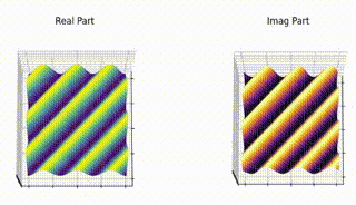
In \(F(k_x, k_y)\) plane stepping through the \(k_x\) and \(k_y\) coordinates creates 2D sinosoids with varying ‘wiggles’ in x and y directions.
Understanding the appearance and behavior of 2D sinusoids in the context of the Fourier Transform requires a closer look at the \(F(k_x, k_y)\) plane. In this plane, navigating through various \(k_x\) and \(k_y\) coordinates generates a series of 2D sinusoids, each characterized by distinct patterns or ‘wiggles’ in both the x and y directions.
The Influence of \(k_x\) and \(k_y\) on Sinusoidal Patterns
Imagine a coded animation, similar to the one in the 1D Fourier transform blog, to better visualize this concept. As you increment the value of \(k_x\), you’ll notice an increase in the frequency of wiggles along the x-direction. Similarly, increasing \(k_y\) boosts the frequency of wiggles in the y-direction. This relationship is key to understanding how 2D sinusoids are formed and manipulated in Fourier space.
Each 2D sinusoid is shaped by a corresponding phasor. This phasor adjusts both the amplitude and phase of the sinusoid. The resultant effect is a versatile range of sinusoidal waves, each uniquely contributing to the overall image reconstruction process in MRI.
The number of wiggles or oscillations in each direction correlates directly to a specific point in the \(F(k_x, k_y)\) plane. For instance, a sinusoid with 3 complete cycles in the x-direction and 3 in the y-direction would correspond to a point in \(F(k_x, k_y)\) with \(k_x =3\) value and \(k_y =3\) value. This mapping is fundamental to how spatial frequencies are represented and manipulated in the Fourier Transform, particularly in applications like MRI, where precise spatial information is crucial.
Here’s a part of animation that demonstrates the relation between point in \(F(k_x, k_y)\) plane and the 2D sinosoid it generates and the effect of phasor assosiated with each of the 2D sinosoid (spatical frequency) and how it scales and shifts the it.
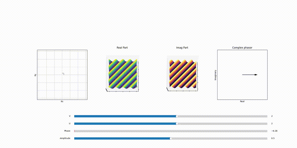
You can play around with the code for this animation on my github repo here.
As a proof of concept, let’s consider a Mario sprite image. We start by taking its Fourier transform, represented as:
\[F(k_x, k_y) = \int_{-\infty}^{\infty} \int_{-\infty}^{\infty} f(x, y) e^{-2\pi i(k_x x + k_y y)} \, dx \, dy\]Here, \(f(x, y)\) is our original Mario sprite image, and \(F(k_x, k_y)\) is its Fourier transform, with \(k_x\) and \(k_y\) representing spatial frequencies in the x and y directions, respectively.
To reconstruct the original image from its Fourier transform, we take each point in the \(F(k_x, k_y)\) plane, which is a complex number (phasor). The reconstruction process involves the following steps:
-
Constructing 2D Sinusoids: For each point \((k_x, k_y)\) in the Fourier transform, we create a corresponding 2D sinusoid in its complex exponential form:
\[S(x, y; k_x, k_y) = e^{2\pi i(k_x x + k_y y)}\] -
Scaling with the Phasor: The phasor at each point in the \(F(k_x, k_y)\) plane, characterized by an amplitude \(A\) and phase \(\phi\), scales the corresponding 2D sinusoid. This scaling is represented as:
\[S_{scaled}(x, y; k_x, k_y) = A \cdot e^{2\pi i(k_x x + k_y y) + \phi}\] -
Summing Spatial Frequencies: The final step involves summing these scaled and shifted sinusoids across all spatial frequencies to reconstruct the original image:
\[f_{reconstructed}(x, y) = \sum_{k_x, k_y} S_{scaled}(x, y; k_x, k_y)\]
This method demonstrates the practical application of Fourier Transform in image processing, showcasing how an image can be decomposed and then reconstructed using the principles of spatial frequencies and phase shifts.
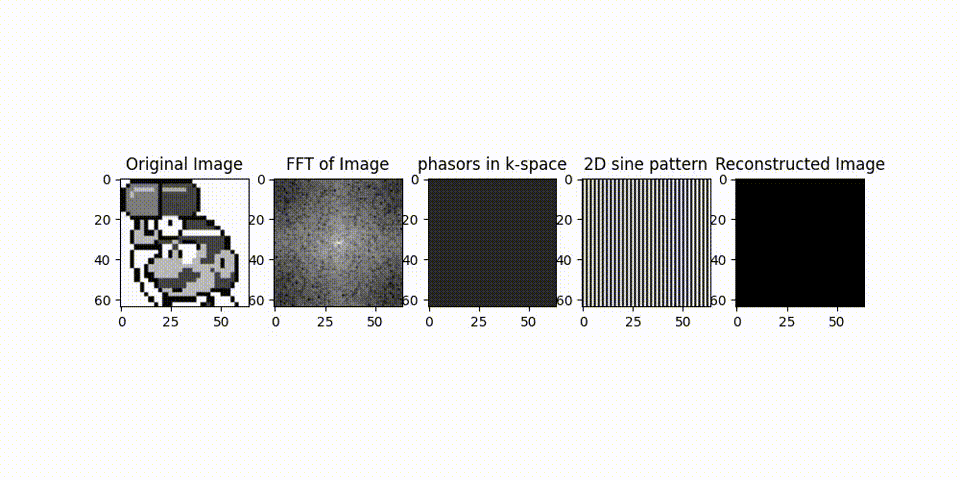
In Fig.3 as we keep adding the 2D sinosoids we get the final image. This is the essence of the Fourier Transform: decomposing a signal into its 2D sine patterns and then reconstructing it from these components.
Share on
Twitter Facebook LinkedInComments are configured with provider: facebook, but are disabled in non-production environments.