
If you haven’t read my previous blog on the relation between complex numbers and rotations, I would highly recommend you to check it out here. It will help you understand the concepts in this blog better.
Introduction
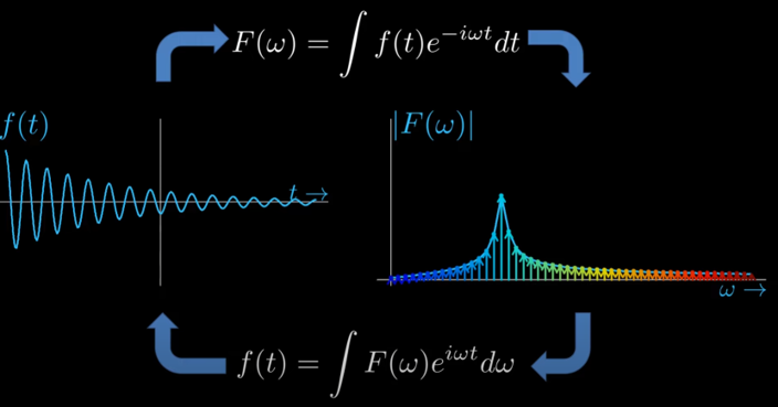
The Fourier Transform is a mathematical tool that transforms a signal from the time domain to the frequency domain, unveiling the different frequencies that constitute the signal. In its most general form, the Fourier Transform is given by:
\[F(\omega) = \int_{-\infty}^{\infty} f(t) e^{-i \omega t} \, dt\]Here, \(F(\omega)\) is the Fourier Transform of \(f(t)\), with \(\omega\) representing frequency and \(t\) denoting time. The exponential term \(e^{-2\pi i \omega t}\) is a rotating complex sinusoid, which is crucial for extracting the frequency components from \(f(t)\).
The Discrete Fourier Transform (DFT)
In digital applications, we use the Discrete Fourier Transform (DFT) to handle sampled data:
\[F(k) = \sum_{n=0}^{N-1} f(n) e^{ i \frac{kn}{N}}\]Here, \(f(n)\) is the sampled signal, \(N\) is the number of samples, and \(k\) is the frequency index in the DFT.
The Discrete Fourier Transform (DFT) is a transformative tool in signal processing, translating signals from the time domain into the frequency domain. While the equations of the Fourier Transform and DFT are familiar territory for many, the real magic lies in understanding what happens inside the DFT and how it reveals the intricate composition of any signal.
Fundamental principle behind fourier transform is that any signal that is changing (temporally or spatially) can be represented as an infinite sum of sinosoids. or in other words we can create any signal by adding different frequencies of sinosoids. This is the basis of fourier transform.
The easiest examples would be temporally varrying 1D signals
Inside DFT
The output of the DFT is a collection of complex numbers, each representing a unique sinusoid in the original signal. These complex numbers, or phasors, hold the key to both the amplitude and phase of these complex sinusoids, essentially encoding how each sinusoid is scaled and shifted.
Complex Phasors
A phasor \(F(\omega = \omega_0)\) in the DFT output is more than just a number; it’s a vector in the complex plane.And in fourier transform plot we mostly show the magnitude of this phasor. For example: Figure 1 illustrates the Fourier Transform and Inverse Fourier Transform of a simple signal. In \(F(\omega)\) plot, the x-axis is the frequency index \(\omega =\omega_0\), while the y-axis is the magnitude of the phasor \(|F(\omega_0)|\).
The magnitude indicates the contribution of each sinusoid to the overall signal.
Thus a phasor \(F(\omega_0)\): \(F(\omega = \omega_0) = x + iy\) with amplitude \(A\): \(A = \sqrt{x^2 + y^2}\) and phase \(\phi\): \(\phi = \tan^{-1}(\frac{y}{x})\)
scales the base complex sinosoid \(e^{- i \omega_0 t}\) by a factor of \(A\) and shifts it by a phase of \(\phi\) \(A e^{- i \omega_0 t + \phi }\)
Each of these sinusoids is a fundamental building block of the orignal signal, characterized by a specific frequency. The DFT decomposes the signal into these basic elements, revealing how each frequency contributes to the overall structure of the signal
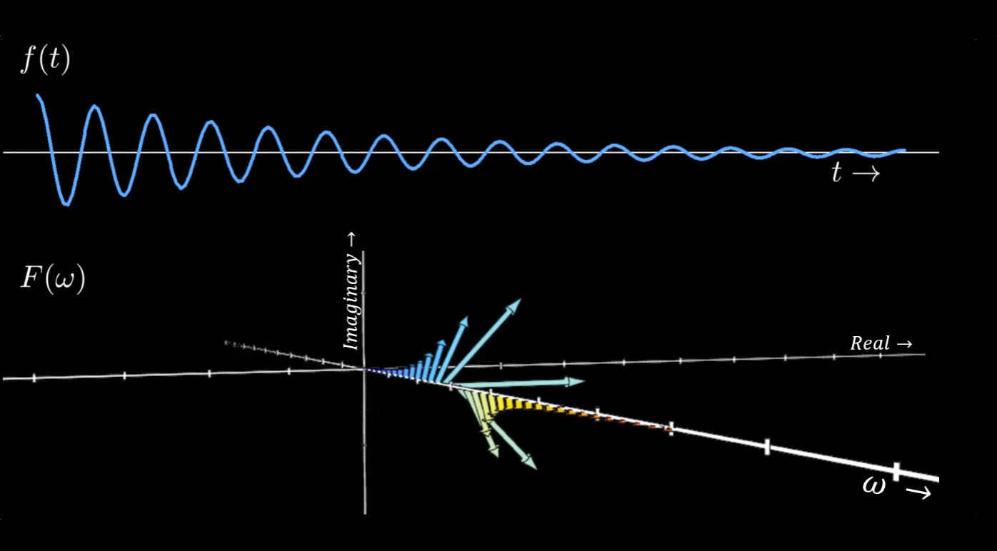
Since each point alone \((\omega)\) in the Figure 1 is a complex number, thus every frequeny \(\omega\) in the \(F (\omega)\) plot has it’s own Argand plane with real and imaginary axis. So we can extend our orignal \(|F(\omega_0)|\)plot from Figure 1 to show that every frequency \(\omega_0\) contains within it a phasor \(F (\omega_0)\) that scales and shifts the sinosoid at \(\omega_0\) according to it’s contribution to the signal.
Sum of Sinusoids
Ultimately, any signal \(f(t)\) can be represented by a specific set of scaled and shifted sinusoids. And Summing over these sinosoids, governed by the principles encoded in the phasors, gives us back the original signal in its time-domain form. This is the essence of the DFT: decomposing a signal into its sinusoidal components and then reconstructing it from these components.
Exploring the DFT with coded Animation
Through animation, we can dynamically illustrate the transformative process of the DFT. The goal is to visually demonstrate how:
Each point in the \(F(\omega)\) plot corresponds to a certain frequency and an associated phasor. These phasors define the amplitude and phase of sinusoids at these specific frequencies. By summing these scaled and shifted sinusoids, we can reconstruct the original signal.
For further exploration and hands on experience I have provided the code for this animation on my github repo here.
This blogpost is a prereq to MRI simulation. These fundamental concepts will help us venture into the realm of 2D Fourier Transforms, K-Spaces and their pivotal role in applications like MRI, opening doors to a world where these concepts find profound applications.
Reference
Share on
Twitter Facebook LinkedInComments are configured with provider: facebook, but are disabled in non-production environments.