Complex Numbers and Rotations: A Primer to Fourier Transform and MR Physics and Simulation

Introduction

Complex numbers often appear mysterious to those who encounter them for the first time. Why would anyone need numbers that are “imaginary”? As it turns out, complex numbers are not only elegant but incredibly useful. They lie at the heart of many scientific and engineering disciplines, including signal processing, control theory, electromagnetism, and, of course, Fourier Transform and Magnetic Resonance (MR) physics.

Complex Numbers and Rotations

Complex numbers and rotations are fundamental to the understanding of the encoding of spatial information. In this Blogpost, we’ll go beyond mere equations and actively code to visualize these concepts. Through this hands-on approach, we’ll deepen our understanding of the core principles involved in not just MR Physics but many other physical concepts that invovle waves, frequencies, phase and rotations. For a more intuivie understanding of complex numbers, I highly recommend 3Blue1Brown’s video on the topic. Here we will write code to visualize the concepts discussed in the video.

What are Complex Numbers?

A complex number \(z\) is defined as \(z = a + bi\), where \(a\) and \(b\) are real numbers, and \(i\) is the imaginary unit with the property \(i^2 = -1\).

\[z = a + bi\]

Plotting Complex Numbers

The Complex Plane

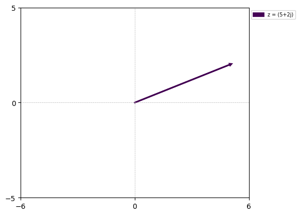
The real part is plotted along the x-axis, and the imaginary part along the y-axis. This 2D plane is known as the complex plane.

from matplotlib import markers
import numpy as np
import matplotlib.pyplot as plt
from matplotlib.animation import FuncAnimation

def plot_arrow(complex_num, xlim=(-2,2),ylim=(-1,1)):
        
    fig, ax = plt.subplots()
    ax.set_xlim(xlim)
    ax.set_ylim(ylim)
    ax.set_aspect('equal')
    plt.grid(True, which='both', axis='both', linestyle='--', linewidth=0.5)
    plt.xticks([np.min(xlim),0,np.max(xlim)])
    plt.yticks([np.min(ylim),0,np.max(ylim)])
    # Define a colormap (cmap) and normalize it
    cmap = plt.get_cmap('viridis')
    norm = plt.Normalize(0, len(complex_num))
    for i in range(len(complex_num)):
        x,y = complex_num[i].real, complex_num[i].imag
        color = cmap(norm(i))

        ax.arrow(0, 0, x, y, head_width=0.1, head_length=0.1, fc=color, ec=color, lw=2)
            # Add a legend

    legends = [f'z = {np.round(z, 2)}' for z in complex_num]
    ax.legend(legends, loc='upper left', bbox_to_anchor=(1, 1), fontsize=7)
    
    
    return fig, ax
    

complex_num = [5+2j]

fig, ax = plot_arrow(complex_num, xlim=(-6,6),ylim=(-5,5))
plt.show()

png

Scaling Complex Numbers

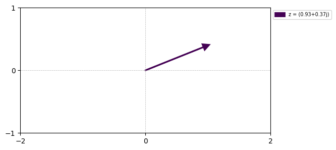
We often need to scale complex numbers to unit magnitude. The magnitude (\(\lVert z \rVert\)) of a complex number \(z = a + bi\) is given by:

\[\lVert z \rVert = \sqrt{a^2 + b^2}\]

# Scaled complex numbers
mag = np.abs(complex_num)
angle = np.angle(complex_num)
scaled_complex_num = 1/mag * complex_num
fig, ax = plot_arrow(scaled_complex_num)

png

Euler’s Formula and Exponential Form of Complex Numbers

One of the most beautiful equations in mathematics is Euler’s formula:

\[e^{ix} = \cos(x) + i \sin(x)\]

This formula allows us to represent complex numbers in exponential form, providing a new way to understand rotation and scaling in the complex plane.

#alternative representation
angle = np.angle(scaled_complex_num)
exponential_form = np.exp(1j * angle)
x, y = np.real(exponential_form), np.imag(exponential_form)
fig, ax = plot_arrow(exponential_form)

png

what if we want to describe rotations?

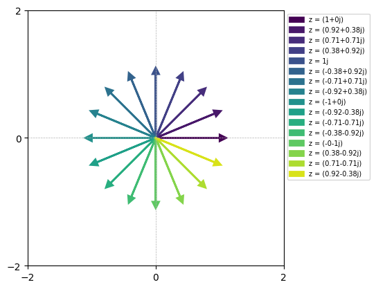
Euler’s formula is a powerful tool for describing rotations in the complex plane. Let’s say we want to rotate a complex number \(z\) by \(\theta\) radians. We can do this by multiplying \(z\) by \(e^{i\theta}\). here we keep the \(z\) to be 1 and vary the theta from 0 to 2pi

# what if we want to describe rotations? 
theta = np.arange(0, 2*np.pi, np.pi/8)
complex_nums = np.exp(1j * theta)
fig, ax = plot_arrow(complex_nums, ylim=(-2,2))
plt.show()

png

Ploting the real and imaginary part of the complex number

# plotting only the real part of the complex number
theta = 2 * np.pi  # 1 rotation
dt = np.arange(0, 5+0.01, 0.01)
complex_num = np.exp(1j * theta * dt)
plt.plot(dt, np.real(complex_num), label='real')
plt.plot(dt, np.imag(complex_num), label='imag')

plt.show()

png

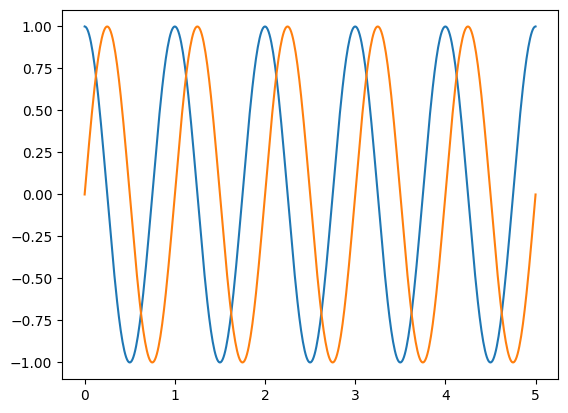
so basically \(e^{ix}=cos(x)+ isin(x)\)

Animation showing how exponential form of complex number can be used to describe rotations in 2D complex plane

import matplotlib.pyplot as plt
from matplotlib.animation import FuncAnimation
import numpy as np
class animate:
    def __init__(self, complex_nums, dt):
        # Figure setup
        self.dt = dt
        self.complex_num = complex_nums
        self.fig, self.ax = plt.subplots()
        self.ax.set_xlim(-2, 2)
        self.ax.set_ylim(-1, 1)
        self.ax.set_aspect('equal')
        plt.grid(True, which='both', axis='both', linestyle='--', linewidth=0.5)
        plt.xticks([-2, 0, 2])
        plt.yticks([-1, 0, 1])

        # Define a colormap (cmap) and normalize it
        cmap = plt.get_cmap('viridis')
        color = cmap(0)
        self.arrow = self.ax.arrow(0, 0, 0, 0, head_width=0.1, head_length=0.1, fc=color, ec=color, lw=2)
        self.legend_text = self.ax.legend([f'z = {np.round(self.complex_num[0], 2)}'], loc='upper left', bbox_to_anchor=(0.5, 1), fontsize=7)
        # Create the legend in the init function

    def init(self):
        self.arrow.set_xy([[0, 0]])  # Initialize arrow at (0, 0)
        return [self.arrow, self.legend_text]

    def update(self,i):
        self.arrow.set_xy([[0, 0], [self.complex_num[i].real, self.complex_num[i].imag]])  # Set arrow's vertices
        # Update the legend text
        self.legend_text.get_texts()[0].set_text(f'z = {np.round(self.complex_num[i], 2)}')
        return [self.arrow, self.legend_text]

    def plot(self):
        anim = FuncAnimation(self.fig, self.update, init_func=self.init, frames=len(self.dt), interval=10, blit=True, repeat=True)
        return anim

theta = 2 * np.pi  # 1 rotation
dt = np.arange(0, 5 + 0.01, 0.01)
complex_num = np.exp(1j * theta * dt)
anim = animate(complex_num, dt)
an = anim.plot()
plt.show()

gif

Changing the direction of rotation

# including a minus sign in the exponential form will result in a rotation in the opposite direction
theta = 2 * np.pi  # 1 rotation
dt = np.arange(0, 5 + 0.01, 0.01)
complex_num = np.exp(-1j * theta * dt)
anim = animate(complex_num, dt)
an = anim.plot()
plt.show()

gif

Inlcude frequency component to the complex number to control the speed of rotation

f = .3  # frequency
theta = 2 * np.pi  # 1 rotation
dt = np.arange(0, 5 + 0.01, 0.01)
complex_num = np.exp(1j * theta *f* dt)   # exp(1j * 2*np.pi* f * t) or exp(1j * omega * dt)

anim = animate(complex_num, dt)
an = anim.plot()
plt.show()

gif

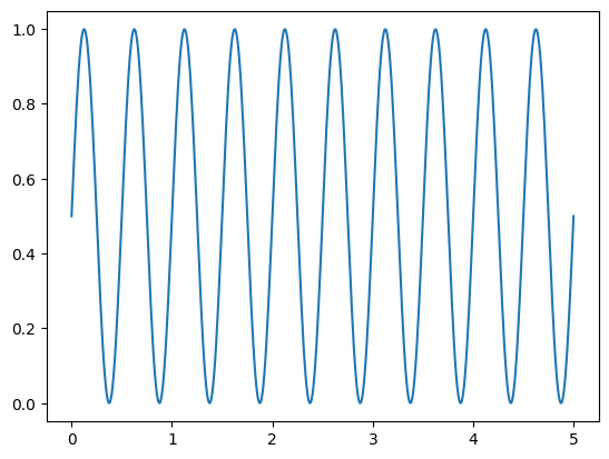
defining a sinonoidal function

# defining a sinonoidal function
g_t = 0.5*np.sin(2 * np.pi * 2 * dt)+0.5
plt.plot(dt, g_t)
plt.show()

png

Scaling the rotations with the function \(g(t)\)

# multiplying the complex number with the function g_t scales the rotating complex number
theta = 2 * np.pi  # 1 rotation
f = .3  # frequency
dt = np.arange(0, 5 + 0.01, 0.01)
complex_num = np.exp(1j * theta *f* dt)*g_t

anim = animate(complex_num, dt)
an = anim.plot()
plt.show()

gif

Why Not Vectors?

At this point, one might wonder, why not use vectors? Vectors can describe points in space and can be scaled and rotated. The answer lies in the algebraic closure of complex numbers and their ability to simplify many mathematical derivations. Complex numbers allow for a unified and elegant representation that turns complicated mathematical operations into simple algebraic ones, especially when it comes to Fourier Transform and MR physics.

The Role of Complex Numbers in Fourier Transform

Fourier Transform breaks down any signal into a sum of sinusoids. In essence, it transforms our signal into a new domain where it’s expressed as a linear combination of exponential functions. This is where complex numbers shine.

\[X(f) = \int_{-\infty}^{\infty} x(t) \cdot e^{-i 2 \pi f t} \, dt\]

The role of complex numbers here is twofold:

The sinusoidal functions are compactly represented using Euler’s formula.
The rotation and scaling properties of complex numbers help in understanding how each frequency component contributes to the overall signal.

Key Takeaways

Complex Plane Representation: Complex numbers can be visualized in a 2D Cartesian coordinate system known as the complex plane. In this plane, the real part serves as the x-axis, while the imaginary part serves as the y-axis.
Scaling and Rotation: Similar to vectors, complex numbers can be scaled and rotated within the 2D complex plane. These operations are particularly useful for understanding various mathematical and physical phenomena.
Exponential Form: Euler’s formula provides an elegant exponential representation for complex numbers. This form is not only mathematically compact but also extremely useful for understanding the rotation and scaling of complex numbers over time.
Trigonometric Components: The rotation of a complex number inherently involves sinusoidal (sine) and cosinusoidal (cosine) components. This is best represented through Euler’s formula, \(e^{ix} = \cos(x) + i\sin(x)\).
Fourier Transform: Understanding these properties of complex numbers is crucial when delving into Fourier Transform. The Fourier Transform essentially decomposes a signal into a series of scaled and rotated complex numbers, which are essentially sinusoids in disguise.

Twitter Facebook LinkedIn