All Things RF Pulse: From Single Wire to Birdcage Coil Simulation
The Magnetic Field Around a Wire: Biot–Savart’s Discovery
In 1820, a simple classroom demonstration changed science: Hans Christian Ørsted noticed a compass needle jump when he switched on an electric current in a wire. This surprise revelation – that electricity can create magnetism – set the stage for a new era in physics. Shortly after, French scientists Jean-Baptiste Biot and Félix Savart took up the mystery. Through careful experiments, they quantified the magnetic field around a current-carrying wire, formulating what we now call the Biot–Savart law. In plain terms, their law says that each tiny segment of current produces a magnetic field that circles around the wire. The strength of this field falls off with distance, and its direction wraps around the wire according to the right-hand rule (point your thumb along the current, and your fingers curl in the field’s direction).
Mathematically, the Biot–Savart law is expressed as an integral:
$$ \mathbf{B}(\mathbf{r}) = \frac{\mu_0}{4\pi} \int_C \frac{I\,d\boldsymbol{\ell} \times \hat{\mathbf{r}}'}{|\mathbf{r}'|^2}\,, $$
where $I,d\boldsymbol{\ell}$ is a current element on the wire path $C$, and $\hat{\mathbf{r}}'$ is a unit vector pointing from that current element to the point $\mathbf{r}$ where we calculate the field. This looks complicated, but for a very long straight wire it simplifies nicely. If a steady current $I$ runs through an infinitely long wire, the magnetic field at a distance $r$ from the wire is:
$$ B(r) = \frac{\mu_0\,I}{2\pi\,r}\,, $$
pointing in circles around the wire (tangent to a circle of radius $r$ around the wire). The $\mu_0$ here is the permeability of free space – a constant that sets the scale of magnetic effects. This formula tells us a crucial fact: electric currents create magnetic fields, and those fields form closed loops around the current.
And if the wire has a finite length then the magnetic field at a point in space is given by
Analytic finite-wire formula
$$ \mathbf B(\mathbf r)=\frac{\mu_0 I}{4\pi R_\perp}\, (\sin\theta_2+\sin\theta_1)\,\hat{\boldsymbol\phi}, $$
where $\theta_1,\theta_2$ are the end-angles subtended at the
for full derivation of this formula, see this video.
Given this background, we can now explore how to compute the magnetic field around a wire in practice, especially in the context of MRI coil simulations.
- Analytic finite-wire formula – exact, fast.
- Numerical line-integral – slower but works for any bent or segmented wire if you refine the sampling.
Each snippet quotes the corresponding Biot–Savart equation inside the comments so you can see how code ↔ math line up.
1 Analytic field of a finite straight wire
For a straight segment from p₁ to p₂ (end-points in 3-D) carrying steady complex current I:
$$ \boxed{\; \mathbf B(\mathbf r)=\frac{\mu_0 I}{4\pi R}\; \bigl(\sin\theta_2+\sin\theta_1\bigr)\, \hat{\boldsymbol\phi}\;} $$
Definitions
- $\mathbf R = \mathbf r - \mathbf r_\text{mid}$ is the vector from the segment centre to the field point; $R = |\mathbf R|$.
- $\theta_1,\theta_2$ are the angles subtended by the extensions of p₁-r and p₂-r to the observation point.
- $\hat{\boldsymbol\phi} = \dfrac{\hat z \times \mathbf R}{R}$ is the azimuthal unit-vector (right-hand rule).
Comments
- Matches the text-book “finite straight conductor” formula.
- Works everywhere except exactly on the wire axis (
R_perp → 0).
import numpy as np
import pyvista as pv
pv.set_jupyter_backend("html") # <- no trame server
from scipy.constants import mu_0
def biot_savart_segment_exact(p1, p2, r_obs, I):
"""
Exact B-field (phasor) of a finite straight wire.
p1, p2 : ndarray (3,), endpoints [m]
r_obs : ndarray (N,3), observation points [m]
I : complex scalar current [A]
returns : ndarray (N,3), complex B-field [T]
"""
# Vector from p1 to p2 (wire direction)
dl = p2 - p1
L = np.linalg.norm(dl) # segment length
dl_hat = dl / L # unit vector along wire
z_hat = dl_hat # choose local z along the wire
# Vectors from ends to observation points
r1 = r_obs - p1 # (N,3)
r2 = r_obs - p2
# Distances
R1 = np.linalg.norm(r1, axis=1)
R2 = np.linalg.norm(r2, axis=1)
# Perpendicular (radial) component magnitude
# R_perp = |r × dl_hat| (distance from wire axis)
R_perp = np.linalg.norm(np.cross(r1, dl_hat), axis=1)
# Angles θ1, θ2 between wire and lines to obs-point
# sinθ = R_perp / R
sin_th1 = R_perp / (R1 + 1e-12)
sin_th2 = R_perp / (R2 + 1e-12)
# Azimuthal unit-vector phî = (dl_hat × r̂)/|dl_hat × r̂| the right hand rule
phi_hat = np.cross(dl_hat, r1) # (N,3) still not unit
phi_hat /= (np.linalg.norm(phi_hat, axis=1)[:, None] + 1e-12)
prefac = mu_0 * I / (4*np.pi*R_perp + 1e-12) # μ0 I / (4π R⊥)
coeff = (sin_th2 + sin_th1) # (N,)
return (prefac * coeff)[:, None] * phi_hat # (N,1)*(N,3)
2 Numerical Biot–Savart line integral
When your wire is bent, segmented, or you just want brute-force fidelity, sample it into small pieces and sum:
$$ \mathbf B(\mathbf r)=\frac{\mu_0}{4\pi}\sum_{j} I\,\frac{\Delta\boldsymbol\ell_j \times (\mathbf r-\mathbf r_j)} {|\,\mathbf r-\mathbf r_j\,|^{3}} . $$
Comments
- Converges to the analytic result as n_steps → ∞.
- Automatically handles wires of arbitrary shape if you break them into straight segments and call this repeatedly.
def biot_savart_segment_numeric(p1, p2, r_obs, I, n_steps=200):
"""
Numerical Biot–Savart integral along a straight segment.
Subdivides the wire into n_steps tiny elements Δℓ.
"""
# Parametric points along the wire
s = np.linspace(0, 1, n_steps, endpoint=False) + 0.5/n_steps
dl = (p2 - p1) / n_steps # tiny segment vector (3,)
# Observation minus mid-point of each sub-segment
r_mid = p1 + np.outer(s, (p2 - p1)) # (n_steps,3)
r_vec = r_obs[:, None, :] - r_mid[None, :, :] # (N, n_steps, 3)
R = np.linalg.norm(r_vec, axis=2)[..., None] # (N, n_steps, 1)
cross = np.cross(dl, r_vec) # (N, n_steps, 3)
dB = mu_0 * I / (4*np.pi) * cross / (R**3 + 1e-18)
return dB.sum(axis=1) # sum over segments
When to use which?
Use the analytic version whenever the segment-length is not comparable to voxel distance (most MRI coil grids). Switch to the numeric version if you need curved wires, end effects, or simply want a ground-truth benchmark.
Additionally, if you want to compute the field around a small segment of wire, you could also use: The integral form of the Biot–Savart law is basically a summation of the contributions from each infinitesimal segment of the wire. For a small segment, we can approximate the field as:
# Biot-Savart function for a straight wire small segment
def biot_savart_segment(p1, p2, r_obs, I):
dl = p2 - p1
r0 = r_obs - (p1 + p2) / 2
norm_r0 = np.linalg.norm(r0, axis=1)[:, np.newaxis] + 1e-12
cross = np.cross(dl, r0)
return mu_0 / (4 * np.pi) * I * cross / (norm_r0**3)
# This script is designed to visualize the magnetic field of a coil using PyVista.
gamma = 42.58e6 # Hz/T for proton
omega = 3 * gamma # Larmor frequency ~128 MHz for 3T for our MAGNETOM Vida Fit scanner
# Compute field from all wires at all observational positions
def compute_field_at_t(wire_actors, obs_positions,L, ti, g_norm=None):
B_total = np.zeros((obs_positions.shape[0], 3), dtype=np.complex128)
for (_, phi, (x, y)) in wire_actors:
I = np.exp(1j * (omega * ti + phi))
p1 = np.array([x, y, -L/2])
p2 = np.array([x, y, L/2])
B = biot_savart_segment_exact(p1, p2, obs_positions, I)
B_total += B
if g_norm is not None:
B_total *= g_norm
return B_total
# Field evaluation grid at center plane
grid_span = 0.2
Ngrid = 50
gx = np.linspace(-grid_span, grid_span, Ngrid)
gy = np.linspace(-grid_span, grid_span, Ngrid)
gx, gy = np.meshgrid(gx, gy)
gz = np.zeros_like(gx)
positions = np.stack([gx.ravel(), gy.ravel(), gz.ravel()], axis=1)
# Parameters
Nr = 1 # Number of wires
L = 0.03 # Length of wires
wire_radius = 0.002 # Thickness of wires
# omega = 0
Nt = 600 # Number of animation frames
t = np.linspace(0, 1e-6, Nt) # Time from 0 to 1 µs
# Spin parameters
M0 = np.array([0, 0, 1]) # Initial magnetization
# Create wire geometry
angles = np.linspace(0, 2*np.pi, Nr, endpoint=False)
wire_positions = np.array([[0,0]]) # Center wire at origin
current_phases = [0] # Phase shift per wire
anim_name = "b1_1_wire.gif"
html = pv_field_animation(
wire_positions,
current_phases,
t,
positions,
anim_name=anim_name,
)
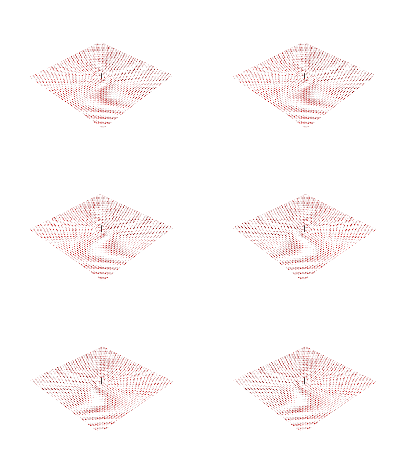
EmbeddableWidget(value='<iframe srcdoc="<!DOCTYPE html>\n<html>\n <head>\n <meta http-equiv="Content-…
Rotating B1 Field Visualization
↳ Source: b1_1_wire.gif.html
One Wire is Not Enough: From Loops to the Birdcage Coil
A single straight wire is neat, but early engineers realized it’s not very efficient at delivering magnetic fields to an entire sample (like a human body). One improvement is to bend the wire into a loop. A loop of current produces a more useful field: inside the loop (along its central axis), the magnetic field lines bunch up and point mostly in one direction (similar to a bar magnet). In fact, the on-axis field of a loop of radius $R$ carrying current $I$ is given by:
$$ B_{\text{on-axis}}(x) = \frac{\mu_0\,I\,R^2}{2(R^2 + x^2)^{3/2}}\,, $$
directed along the loop’s axis. At the center of the loop ($x=0$), this simplifies to $B = \frac{\mu\_0 I}{2R}$ along the axis. So a loop concentrates the field in a specific region – a handy trait for an RF coil in MRI, which needs to bathe the tissue in a strong magnetic RF field. Early NMR experiments in the 1940s (by pioneers like Felix Bloch and Edward Purcell) often used loop-like coils to transmit and receive signals. They knew that sending a radiofrequency pulse through such a coil could tip the tiny “magnetization” of nuclei and detect it – the birth of NMR and eventually MRI.
Magnetic field created through a loop is shown in the figure below. This is a classic textbook example of a magnetic field around a current-carrying loop. The field lines are denser inside the loop, indicating a stronger magnetic field there.
Magnetic field around a current-carrying loop
</img>Spin Excitation and Transverse
To stimulate the NMR spin system, an RF-coil must produce a time-varying excitation field B1(t) with the following characteristics:
✔ B1(t) must have components that rotate near the resonant frequency (ωo), and
✔ B1(t) must have components perpendicular to the static magnetic field (Bo)
The simplest form of such an RF-transmit coil is a single loop oriented at right angles to the main magnetic field (see figure right). By driving a sinusoidal alternating current through this loop at the Larmor frequency, an oscillating magnetic field perpendicular to Bo is produced. Somewhat more sophisticated variations of this coil can be easily imagined, such as 2-loop (Helmholz) or multi-loop (solenoid) configurations.
Magnetic field around a current-carrying loop
Linearly Polarized Fields and Counter-Rotating Decomposition
What kind of field excites NMR?
To excite nuclear spins efficiently, the transmit RF field B₁(t) must satisfy two physical constraints:
$$ \begin{aligned} &\textbf{(i)}\quad B_1(t)\;\perp\;B_0\quad &\text{(must be transverse)}\\ &\textbf{(ii)}\quad B_1(t)\;\text{rotates at } \omega_0 \quad &\text{(must match Larmor frequency)} \end{aligned} $$
Consider the nuclear magnetisation vector $\vec{M}$ in a rotating frame. The Bloch equation tells us that only the component of the RF field that co-rotates with $\vec{M}$ at the Larmor frequency contributes to tipping it:
$$ \frac{d\vec{M}}{dt} = \gamma\,\vec{M} \times \big[B_0\,\hat{z} + 2\,\Re\{B_1^{+}(t)\,\hat{x}_\text{rot}\} \big] $$
Simulating the LP field and decomposition using two wires π apart
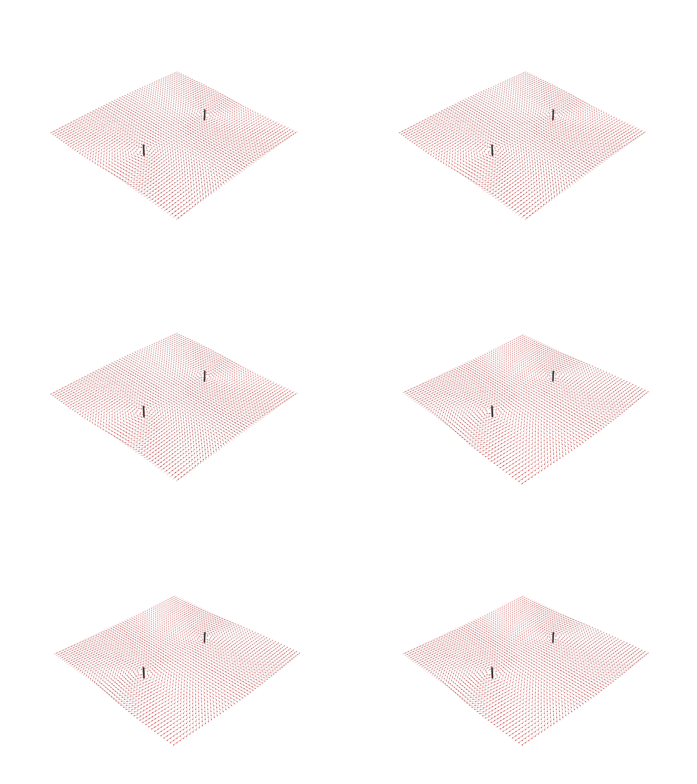
Let’s simulate a minimal LP configuration: two long wires placed π radians apart on a circle, both carrying in-phase current. This is like a simplified Helmholtz pair, producing a transverse oscillating B₁ field along a fixed axis.
This setup approximates a linear-polarized coil with a B₁ field along x.
leak = np.linalg.norm(B1_minus) / np.linalg.norm(B1_plus)
print(f"Fractional B1- leak (LP drive): {leak:.2%}")
You should see:
Fractional B1- leak (LP drive): 100.00%
This confirms the equal-magnitude counter-rotating decomposition of a linearly oscillating field. It's a real physical effect — the field itself is oscillating, but only half of it can rotate with the spins and drive NMR transitions.
When “just two wires” won’t cut it
Two wires driven in-phase → linearly polarized field → 50% wasted energy
Decomposition shows equal $B_1^+$ and $B_1^-$ components
Efficient MRI excitation demands a rotating field — achieved by
- adding a second coil orthogonal and 90° shifted, or
- building a proper birdcage or quadrature array
# Parameters
N_rungs = 2
R = 0.1
Nt = 600
t = np.linspace(0, 0.1e-6, Nt) # Time from 0 to 200 µs
# Geometry: positions of rungs
angles = np.linspace(0, 2*np.pi, N_rungs, endpoint=False)
x_rungs = R * np.cos(angles) # x-coordinates of rungs
y_rungs = R * np.sin(angles) # y-coordinates of rungs: shape (N_rungs,)
# Phase shifts for each rung
current_phases = angles # mode-1 in-phase current i.e no delay in current
wire_positions = np.stack([x_rungs, y_rungs], axis=1) # Center wire at origin
anim_name = "b1_2_rungs_in_phase.gif"
pv_field_animation(
wire_positions,
current_phases,
t*10, # Cscale the time to see animation faster
positions,
anim_name=anim_name,
)
EmbeddableWidget(value='<iframe srcdoc="<!DOCTYPE html>\n<html>\n <head>\n <meta http-equiv="Content-…
# Usage:
pretty_iframe(f"{anim_name}.html", title="2 Wires Field Visualization")
2 Wires Field Visualization
↳ Source: b1_2_rungs_in_phase.gif.html
pretty_gif(anim_name)
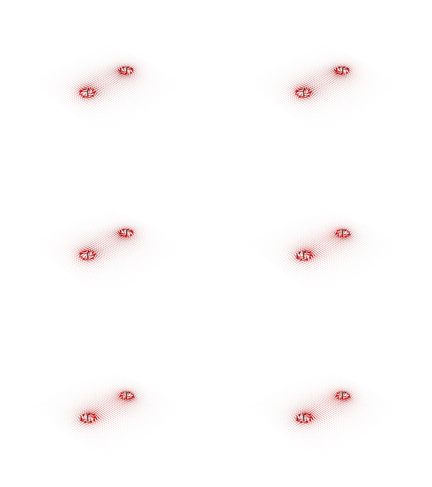
Scaled Magnetic Field Simulation
anim_name = "b1_2_rungs_in_phase_scaled.gif"
pv_field_animation(
wire_positions,
current_phases,
t*10, # Cscale the time to see animation faster
positions,
scaled=True,
anim_name=anim_name,
)
EmbeddableWidget(value='<iframe srcdoc="<!DOCTYPE html>\n<html>\n <head>\n <meta http-equiv="Content-…
pretty_gif(anim_name)
A linearly polarized field is inherently inefficient
Suppose we drive a single loop (or equivalently two opposite wires) with a sinusoidal current:
$$ I(t) = I_0 \cos(\omega_0 t) $$
The resulting magnetic field at the center is also linearly polarized:
$$ \vec{B}_1(t) = B_0 \cos(\omega_0 t)\, \hat{x} $$
But this can be algebraically decomposed into two counter-rotating circular fields:
$$ \boxed{ \vec{B}_1(t) = \frac{B_0}{2}\left[\hat{x} + i\hat{y}\right] e^{-i\omega_0 t} + \frac{B_0}{2}\left[\hat{x} - i\hat{y}\right] e^{+i\omega_0 t} = B_1^+(t) + B_1^-(t) } $$
Here:
- $B_1^+$ rotates with the spin precession (resonant)
- $B_1^-$ rotates against it (off-resonant → ignored)
Because only $B_1^+$ contributes to excitation, 50% of the transmitted power is wasted in a linear coil. Yet, this is the default field generated by many simple configurations.
B_total = np.zeros((2500, 3), dtype=np.complex128)
for φ, (x, y) in zip(current_phases, wire_positions):
I = np.exp(1j * φ) # current phasor
p1 = np.array([x, y, -L/2])
p2 = np.array([x, y, +L/2])
B_total += biot_savart_segment_exact(p1, p2, positions, I)
# Compute B1+ and B1- from complex transverse field
Bx, By = B_total[:, 0], B_total[:, 1]
B1_plus = 0.5 * (Bx + 1j * By)
B1_minus = 0.5 * (Bx - 1j * By)
# Now compute |B1+| map
B1_magnitude = np.abs(B1_plus) # shape = (2500,)
leak = np.linalg.norm(B1_minus) / np.linalg.norm(B1_plus)
print(f"Fractional B1- leak (LP drive): {leak:.2%}")
Fractional B1- leak (LP drive): 100.00%
# Assume you have (x, y) coordinates corresponding to each point
# obs_positions is (2500, 3)
x = positions[:, 0]
y = positions[:, 1]
# Create a 2D scatter or interpolate to a grid
import matplotlib.pyplot as plt
plt.figure(figsize=(5, 5))
plt.scatter(x, y, c=B1_magnitude, cmap='viridis', s=10)
plt.colorbar(label='|B1+| (T)')
plt.title('B1+ Field Map')
plt.xlabel('x (m)')
plt.ylabel('y (m)')
plt.axis('equal')
plt.show()
B1_grid = B1_magnitude.reshape(50, 50)
plt.imshow(B1_grid, extent=[x.min(), x.max(), y.min(), y.max()], origin='lower', cmap='viridis')
plt.colorbar(label='|B1+|')
plt.title('B1+ Field Map')
plt.xlabel('x (m)')
plt.ylabel('y (m)')
Text(0, 0.5, 'y (m)')
This confirms the equal-magnitude counter-rotating decomposition of a linearly oscillating field. It's a real physical effect — the field itself is oscillating, but only half of it can rotate with the spins and drive NMR transitions.
Transverse Magnetic Field: The Birdcage Coil
As we saw, a single loop or linearly polarized coil still has limitations. The field it produces might be strong at the center, but it falls off near the edges. Also, a simple loop’s field can be non-uniform across a large object. And it wastes 50% of the energy as well. To image larger volumes (like a human torso) and to get a uniform excitation, engineers needed a more sophisticated design. This is where the birdcage coil comes in – a design that looks like its namesake and revolutionized MRI in the 1980s.
In 1985, Cecil E. Hayes and colleagues at GE introduced the birdcage resonator. Picture a birdcage: it has two circular end-rings connected by a number of straight bars (the “rungs”) going down the sides radioeng.cz. The MRI birdcage coil is exactly that: two conductive loops (end-rings) and an even number of straight wires (rungs) connecting them. Typically there might be 8, 12, or 16 rungs spaced evenly around a cylinder. Each rung carries current, and capacitors (strategically placed either in the rungs or end-rings) help tune the coil to the desired frequency. The result is a resonant structure that can create a very uniform magnetic field in its center. The name “birdcage” really comes from its appearance.
Birdcage coil design
</img>Visualizing the Current in the Rungs
Let's consider a birdcage coil with N rungs, each carrying a steady current I. First, let's just focus on the Current in the rungs, ignoring the resultant magnetic field for now. If we assume all rungs carry the same current I in the same direction.
# Parameters
N_rungs = 8
R = 0.1
Nt = 600
t = np.linspace(0, 0.1e-6, Nt) # Time from 0 to 200 µs
Angular Position of Each Rung
we are going to place the N_rungs rungs evenly around a circle. The angular position of each rung can be calculated as:
$$\theta_j = \frac{2\pi j}{N_{\text{rungs}}}\,,
$$
where $j$ is the rung index (from 0 to $N_{\text{rungs}}-1$).
Starting the phase $\phi_j$ of the AC current in each rung is set to zero, meaning all rungs are in phase. The current in each rung can be expressed as: $$ I_j = I \cdot e^{i\omega t + \phi_j} = I \cdot e^{i\omega t + 0} = I \cdot e^{i\omega t}, $$ where $I$ is the magnitude of the current in each rung.
# Geometry: positions of rungs
angles = np.linspace(0, 2*np.pi, N_rungs, endpoint=False)
x_rungs = R * np.cos(angles) # x-coordinates of rungs
y_rungs = R * np.sin(angles) # y-coordinates of rungs: shape (N_rungs,)
# Phase shifts for each rung
phases = np.zeros_like(angles) # mode in-phase current i.e no delay in current
from matplotlib.animation import FuncAnimation
import matplotlib.pyplot as plt
from IPython.display import HTML
# Setup figure
fig = plt.figure(figsize=(12,6))
ax_current = fig.add_subplot(1, 1,1)
ax_current.set_xlim(-1.5*R, 1.5*R)
ax_current.set_ylim(-1.5*R, 1.5*R)
ax_current.set_aspect('equal')
lines = [ax_current.plot([], [], lw=3)[0] for _ in range(N_rungs)]
ax_current.set_title("Rotating Current Pattern (Quadrature Drive)")
ax_current.set_xticks([])
ax_current.set_yticks([])
# Animation update function
def update(i):
for j, line in enumerate(lines):
I = 1*np.cos(omega * t[i] + phases[j]) # Current at time t[i] for rung j
# Represent current as color intensity and vector length
x = x_rungs[j]
y = y_rungs[j]
dx = 0.05 * I * np.cos(angles[j])
dy = 0.05 * I * np.sin(angles[j])
line.set_data([x - dx, x + dx], [y - dy, y + dy])
line.set_color(plt.cm.plasma((I + 1)/2)) # map current to color
return lines
ani = FuncAnimation(fig, update, frames=Nt, interval=5,
blit=True,
repeat=True)
plt.close() # Close the figure to avoid displaying it in Jupyter
HTML(ani.to_jshtml())
# ani.save("anim1.gif", writer="ffmpeg", fps=30)
# pretty_gif("anim1.gif", caption="")
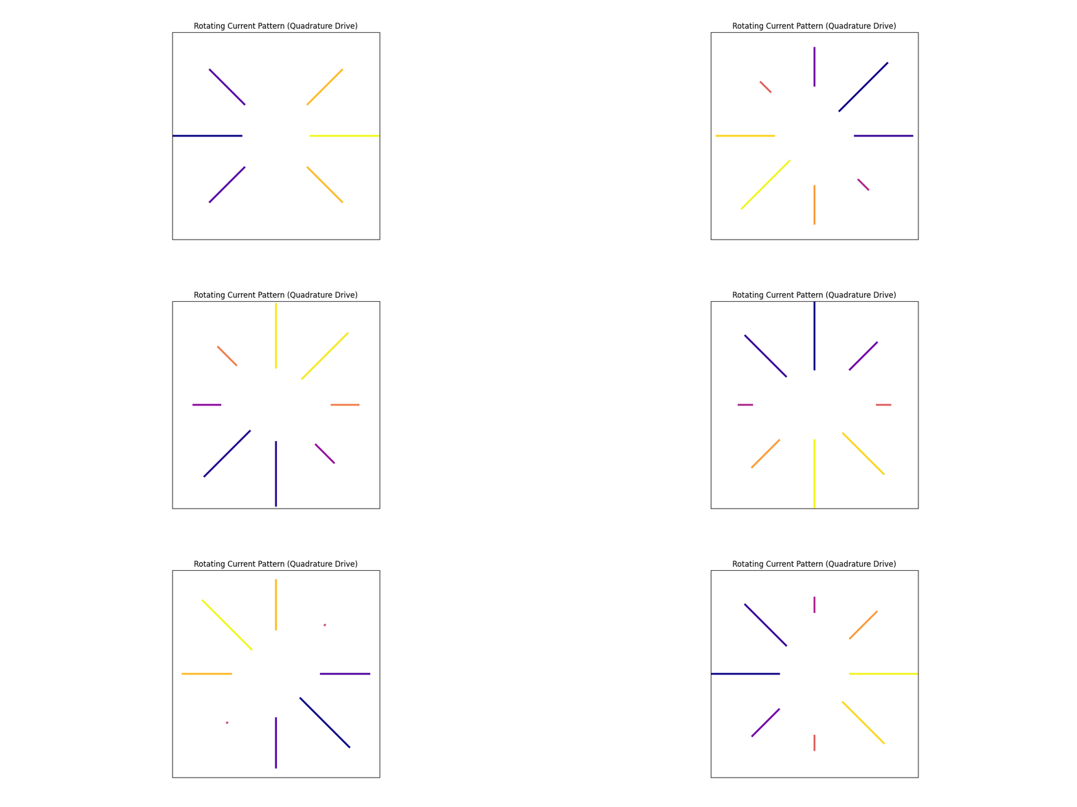
As we can see in the animation above, the current in each rung is represented as a vector rotating around the circle. The length of each vector represents the magnitude of the current, and the color represents its value which are oscillating from positive to negative. Since all rungs have in-phase current $I \cdot e^{i\omega t + 0} $ , they all oscillate in phase.
# Create wire geometry
angles = np.linspace(0, 2*np.pi, N_rungs, endpoint=False)
wire_positions = np.stack([x_rungs, y_rungs], axis=1) # Center wire at origin
current_phases = np.zeros_like(angles) # Phase shift per wire
# current_phases= np.zeros_like(current_phases) # Set all phases to zero for simplicity
# PyVista plotter setup
Now using our knowledge of the Biot-Savart law, we can compute the magnetic field $ \mathbf B(\mathbf r) $ produced by each rung at different grid points in space. and summing them up to get the total magnetic field. $ \mathbf B_{total}(\mathbf r) $
In code, we can implement this as follows:
def compute_field_at_t(B_total,wire_actors, obs_positions,L, ti):
for (_, phi, (x, y)) in wire_actors:
I = np.exp(1j * (omega * ti + phi))
p1 = np.array([x, y, -L/2])
p2 = np.array([x, y, L/2])
B = biot_savart_segment_exact(p1, p2, obs_positions, I)
B_total += B # summing the contributions from each rung for the observation points
return B_total
This function computes the magnetic field at various observation points by iterating over each rung, calculating its contribution using the Biot-Savart law, and summing these contributions to get the total field.
anim_name = "b1_8_rungs_in_phase.gif"
pv_field_animation(
wire_positions,
current_phases,
t*10, # Cscale the time to see animation faster
positions,
anim_name=anim_name,
)
EmbeddableWidget(value='<iframe srcdoc="<!DOCTYPE html>\n<html>\n <head>\n <meta http-equiv="Content-…
# Usage:
pretty_iframe(f"{anim_name}.html", title="Rotating B1 Field Visualization with 8 Rungs")
Rotating B1 Field Visualization with 8 Rungs
↳ Source: b1_8_rungs_in_phase.gif.html
pretty_gif(anim_name)
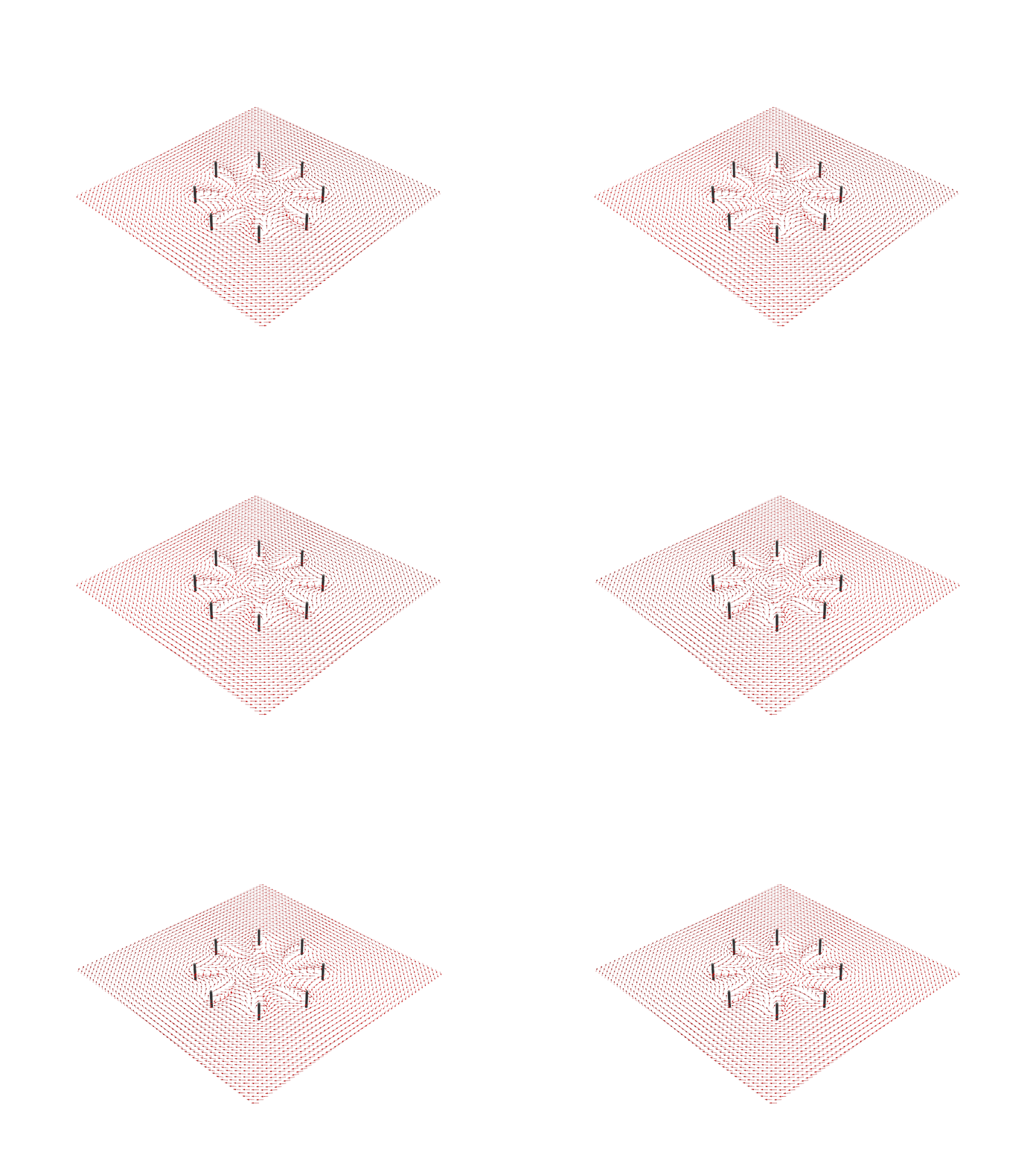
As we can see in the animation above, If all 8 rungs carry the same oscillating current (peaking at the same time), each one generates a magnetic field looping around it. At the centre of the coil, the contributions from these rungs can be added as vectors (using the superposition principle). Intuition might say that by symmetry, the fields could cancel out at dead centre – and indeed, a perfectly symmetric current distribution in the rungs alone produces zero net field at the exact centre if the phases are identical. You can imagine four pairs of opposite rungs whose fields oppose each other. In practice, the “all in-phase” mode of a birdcage coil does not create a strong, uniform transverse field in the centre; This mode is generally not used for MRI excitation (it doesn’t tip the magnetisation). So, in-phase currents alone won’t solve our problem of creating a dynamic, rotating field. We need a twist – quite literally a twist in phase as we go around the coil and the complete current path through the end-rings.
Phase shifts for quadrature drive
The birdcage coil’s magic lies in phasing the currents in each rung. Instead of all rungs peaking together, we feed each successive rung with a slight delay in phase. For an 8-rung coil, this phase increment is 360°/8 = 45° between neighboring rungs. That means if the first rung’s current peaks now, the next rung’s current will peak a tiny fraction of a second later (45° of the RF cycle later), and so on around the circle. In general, for $N$ rungs we use a phase progression of 360°/$N$ per step. This creates what engineers call a traveling wave of current around the cylinder’s circumference. At any given instant, the currents aren’t all equal – one rung might be at maximum current, the next one slightly less, and so forth, in a sinusoidal pattern around the ring. A moment later, the peak current has “moved” to the next rung, and so on, effectively rotating around the coil.
Let's now visualize the quadrature drive, where the currents in adjacent rungs are 90 degrees out of phase.
phases = angles
ani = FuncAnimation(fig, update, frames=Nt, interval=5,
blit=True,
repeat=True)
ani.save("anim2.gif", writer="ffmpeg", fps=30)
pretty_gif("anim2.gif", caption="Rotating Current Pattern (Quadrature Drive)")
Rotating Current Pattern (Quadrature Drive)
# visualize the current pattern
current_plot = plt.figure(figsize=(16, 8))
curr_ax = current_plot.add_subplot(1, 1, 1)
# curr_ax.set_xlim(-1.5, 1.5)
# curr_ax.set_ylim(1, 1.5)
# curr_ax.set_aspect('equal')
curr_ax.set_xticks(np.linspace(0, t.max(), 10))
curr_ax.set_ylabel("Current Magnitude")
curr_ax.set_xlabel("time")
for j in range(N_rungs):
I = 1 * np.cos(omega * t + phases[j]) # Initial current
curr_ax.plot(t, I.real)
curr_ax.legend(phases* 180/(np.pi))
plt.show()
The Resultant Magnetic Field: Rotating in Space
Now consider the magnetic field produced by these phased currents. Each rung still produces its local looping field, but now the peaks of those fields also rotate in time. At the center of the coil, the contributions from all rungs combine to create a net field that rotates in space. For example, imagine a 6-rung coil (to make the phases easy: 60° steps). At time $t=0$, rung 1 has peak current and produces a field pointing, say, “north” in the transverse plane. A bit later, rung 2 peaks, producing a field pointing “northeast.” Then rung 3 peaks (east), rung 4 (southeast), and so on. The superposition of all six contributions at any instant yields a single resultant field in the center. As each rung takes its turn peaking, that resultant field sweeps around like the hand of a clock. In the case of an 8-rung coil with 45° phase steps, the combined field vector in the center will make a full rotation of 360° during one cycle of the RF oscillation.
# Create wire geometry
angles = np.linspace(0, 2*np.pi, N_rungs, endpoint=False)
wire_positions = np.stack([x_rungs, y_rungs], axis=1) # Center wire at origin
current_phases = angles # Phase shift per wire
anim_name = "b1_8_rungs_out_phase.gif"
pv_field_animation(
wire_positions,
current_phases,
t*10, # scale the time to see animation faster
positions,
anim_name=anim_name,
)
EmbeddableWidget(value='<iframe srcdoc="<!DOCTYPE html>\n<html>\n <head>\n <meta http-equiv="Content-…
# Usage:
pretty_iframe(f"{anim_name}.html", title="Rotating B1 Field with 8 Rungs with phase shift")
Rotating B1 Field with 8 Rungs with phase shift
↳ Source: b1_8_rungs_out_phase.gif.html
pretty_gif(anim_name)
Let’s put some math to that intuition. Suppose each rung $k$ (where $k=0,1,2,...,7$ for eight rungs) carries a current $I_k(t) = I_0 \cos(\omega t + \phi_k)$, with phase $\phi_k = k \times 45°$. The magnetic field contribution at the center from rung $k$ can be represented as a vector $\mathbf{b}_k(t)$ in the transverse (x–y) plane. We can write this contribution (up to a proportionality constant) as:
$$ \mathbf{b}_k(t) = b_0 \cos(\omega t + \phi_k)\,\hat{\mathbf{e}}_{\perp}(\phi_k)\,. $$
Here $\hat{\mathbf{e}}*{\perp}(\phi_k)$ is a unit vector pointing perpendicular to rung $k$ (the direction of the field from that rung at the center). Essentially, $\hat{\mathbf{e}}*{\perp}(\phi_k)$ points $90°$ ahead of the rung’s position angle $\phi_k$ (by the right-hand rule). Now, if we sum up all 8 rungs, the total field at the center is:
$$ \mathbf{B}_{\text{total}}(t) = \sum_{k=0}^{7} \mathbf{b}_k(t)\,. $$
When the phases are progressive (by 45°) as described, this sum within the circular rungs simplifies beautifully. All the terms combine to produce something close to:
$$ \mathbf{B}_{\text{total}}(t) \approx B_1 \big[\cos(\omega t)\,\hat{\mathbf{x}} + \sin(\omega t)\,\hat{\mathbf{y}}\big]\,, $$
which is a field of constant magnitude $B_1$ rotating in the x–y plane at angular frequency $\omega$. In other words, by driving the coil rungs in the right phase sequence, we get a circularly polarized magnetic field in the center. The field vector smoothly rotates around, like a lighthouse beam sweeping the horizon – except this “beam” is magnetic and it’s rotating millions of times per second (at the MRI radiofrequency).
This rotating transverse field is often called the B₁ field in MRI. Specifically, we call it the B₁⁺ field when it rotates in the same direction as the precession of nuclear spins (more on that soon). Historically, creating such a rotating field was a big deal. Early MRI systems often used two orthogonal coils driven 90° out of phase (a quadrature coil) to achieve a similar effect – yielding about 40% higher signal-to-noise than a single coil, because the field was used more efficiently. The birdcage coil generalized that idea, using many elements to produce a very homogeneous rotating field. By the late 1980s, virtually all MRI scanners adopted birdcage-style volume coils for body imaging. The result: a strong, uniform RF field that can tip spins effectively.
Larmor Precession: Tuning into the Spinning Nuclei
Why do we care so much about having a rotating magnetic field in the first place? The reason lies at the heart of NMR: nuclear spins behave like tiny magnets that precess (wobble) around the main magnetic field. If the scanner’s main field (B₀) is along (say) the z-axis, then a proton’s magnetization vector will precess around z at the Larmor frequency $\omega_0 = \gamma B_0$, where $\gamma$ is the gyromagnetic ratio (for protons, $\gamma \approx 2\pi \times 42.58$ MHz/T). This precession is like a spinning top circling around the vertical direction. For a 1.5 T scanner, $\omega_0$ is about $2\pi \times 64$ MHz (i.e., about 64 million rotations per second).
Now, to tip over the spin (i.e. to flip the magnetization away from the z-axis into the transverse plane), we need to apply a magnetic field that exerts a torque on it. According to basic physics (the torque equation for a magnetic dipole), a magnetic field that is perpendicular to the spin’s magnetization can push it over. If we apply a static transverse field, the spin will start to precess around the resultant field (which becomes a tilted combination of B₀ and the transverse field). That’s not very efficient or easy to control. Instead, the trick discovered by early NMR pioneers is to apply an oscillating transverse field at the same frequency as the spin’s precession – in other words, on resonance. This is the RF pulse: a magnetic field oscillating at $\omega_0$ applied perpendicular to B₀.
But here’s the key: the field should not only oscillate at the right frequency, it should also rotate in the same sense as the spin’s precession. In our two wire example where we simulated a linearly polarized field, we had a magnetic field oscillating at $\omega_0$ however we saw that the 50% of the magnetic field with opposite rotating component is being wasted away. Since in a linearly oscillating field Half the time it’s pushing the spin in the right direction, and half the time it’s pushing opposite. The net effect is that only half of the power is effectively used to tip the spin, and the other half just cancels out (or worse, can cause unwanted heating). This is why a circularly polarized (rotating) B₁ field is so much more efficient – it’s always pushing the spin “on resonance” and in the correct orientation. A co-rotating field is essentially a resonant driver for the precessing spins.
Thus, we define B₁⁺ to be the rotating magnetic field component that matches the spin precession (the useful part), and B₁⁻ to be the opposite component (the useless part, for excitation). In a linearly polarized coil, the transmit field is split evenly into B₁⁺ and B₁⁻, meaning half the RF power is wasted and does nothing but heat the tissue. In a circularly polarized (quadrature) coil, on the other hand, ideally all the transmit field is B₁⁺ (and $B₁^{-}\approx0$). This is exactly what our phased 8-wire birdcage coil achieves: it generates a transverse field that is (to the extent possible) purely rotating in one direction. As a result, every bit of that field can interact with the nuclear spins and tip them.
Imagine trying to push a child on a merry-go-round. If you push at random times, or opposite to the rotation, you won’t get far. But if you run alongside and give a push exactly as the child comes by, you’ll impart energy efficiently and make the merry-go-round spin faster. In the same way, if our RF magnetic field rotates in sync with the nuclear spin, it continuously nudges the spin in the same direction, accumulating the tipping action.
Historical note: The use of circular polarization in NMR/MRI was quickly adopted once its benefits were understood. Not only does it improve efficiency, but receive coils in quadrature also gain a $\sqrt{2}$ signal boost. The language of “B₁⁺” and “B₁⁻” came later as high-field MRI (e.g. 3 T and above) made B₁ inhomogeneities more pronounced and engineers needed to precisely measure and address the effective driving field in the body. It’s now standard to distinguish the transmit field (B₁⁺) from the receive sensitivity (B₁⁻) when calibrating scanners and designing RF pulses.
Scaled Rotating Magnetic Field Simulation
anim_name = "b1_8_rungs_out_phase_scaled.gif"
pv_field_animation(
wire_positions,
current_phases,
t*10, # Cscale the time to see animation faster
positions,
scaled=True,
anim_name=anim_name,
)
EmbeddableWidget(value='<iframe srcdoc="<!DOCTYPE html>\n<html>\n <head>\n <meta http-equiv="Content-…
pretty_iframe(f"{anim_name}.html", title="Scaled Rotating B1 Field with 8 Rungs wiht phase shift")
Scaled Rotating B1 Field with 8 Rungs wiht phase shift
↳ Source: b1_8_rungs_out_phase_scaled.gif.html
pretty_gif(anim_name)
B_total = np.zeros((2500, 3), dtype=np.complex128)
for φ, (x, y) in zip(current_phases, wire_positions):
I = np.exp(1j * φ) # current phasor
p1 = np.array([x, y, -L/2])
p2 = np.array([x, y, +L/2])
B_total += biot_savart_segment_exact(p1, p2, positions, I)
# Compute B1+ and B1- from complex transverse field
Bx, By = B_total[:, 0], B_total[:, 1]
B1_plus = 0.5 * (Bx - 1j * By)
# Now compute |B1+| map
B1_magnitude = np.abs(B1_plus) # shape = (2500,)
# Assume you have (x, y) coordinates corresponding to each point
# obs_positions is (2500, 3)
x = positions[:, 0]
y = positions[:, 1]
# Create a 2D scatter or interpolate to a grid
import matplotlib.pyplot as plt
plt.figure(figsize=(5, 5))
plt.scatter(x, y, c=B1_magnitude, cmap='viridis', s=10)
plt.colorbar(label='|B1+| (T)')
plt.title('B1+ Field Map')
plt.xlabel('x (m)')
plt.ylabel('y (m)')
plt.axis('equal')
plt.show()
🔁Reshape into a 2D grid
B1_grid = B1_magnitude.reshape(50, 50)
plt.imshow(B1_grid, extent=[x.min(), x.max(), y.min(), y.max()], origin='lower', cmap='viridis')
plt.colorbar(label='|B1+|')
plt.title('B1+ Field Map')
plt.xlabel('x (m)')
plt.ylabel('y (m)')
Text(0, 0.5, 'y (m)')
As we can see from the map above, the magnetic field withing the circular rungs is uniform and has a constant magnitude. However, the field strength decreases as we move away from the center of the coil. The field withing the circular rungs is mostly pure $B_1^+$, which is the rotating component that excites the spins.
🔬 What Above map shows
This B₁⁺ map is what you’d feed into:
Flip angle estimation: α = γ ∫ |B₁⁺(t)| dt
SAR calculation (if conductivity & tissue models available)
RF pulse design (spokes, pTx, etc.)
Shaping the RF Pulse: Sinc Envelopes and Spatial Selectivity
So far, we’ve focused on the geometry of the coil and the polarization of the RF field. We now have a coil (the birdcage or similar) that can generate a B₁⁺ field – a rotating magnetic field – that effectively tips spins. The next part of the story is how we shape this RF field in time to achieve specific goals in imaging. Simply turning on a constant RF field for a certain duration will tip the magnetization by a certain angle (the flip angle). In fact, if you have a field $B\_1$ (in Tesla) on resonance, the flip angle $\theta$ (in radians) is $\theta = \gamma \int B\_1^+(t),dt$. For a constant amplitude, this simplifies to $\theta = \gamma B\_1,\tau$, where $\tau$ is the pulse duration. For example, to achieve a 90° flip (π/2 radians), you’d apply the RF until $\gamma B\_1 \tau = \pi/2$. This might be a few hundred microseconds for typical B₁ strengths in MRI.
However, MRI usually needs slice selection or other spatially selective excitation. This is done by applying a magnetic field gradient at the same time as the RF pulse. The gradient makes the resonance frequency position-dependent (Larmor frequency becomes $\omega(z) = \gamma [B_0 + G ,z]$ for a gradient $G$ along $z$). Then, by shaping the frequency content of the RF pulse, we can excite only spins in a certain slice of the body. How do we shape the frequency content? By modulating the RF amplitude (and phase) as a function of time – essentially designing the pulse’s waveform.
The most famous RF pulse shape in MRI is the sinc pulse. A sinc(x) function in time has a rectangular (brick-wall) shape in frequency space. So if we want to excite a narrow band of frequencies (corresponding to a slice of certain thickness), we use a sinc-modulated RF pulse. In practice, this means the RF is turned on with an amplitude that rises and falls following a sinc envelope (oscillating at the carrier frequency $ω\_0$ underneath). Mathematically, it can be shown that the ideal RF excitation to uniformly cover a given frequency band is indeed a sinc(t) waveform. The “main lobe” of the sinc covers the desired band, and the side lobes (which we try to minimize or truncate) cause ripple or slight excitation outside the band. Typically, scanners use a time-limited sinc (with a few lobes) and often apodize it (taper the edges) to reduce ringing. The end result is an RF pulse that might last a few milliseconds and has a smooth envelope that looks like a sinc function. During this pulse, a slice-select gradient is on, so only spins in the slice whose Larmor frequencies fall under the pulse’s spectrum get flipped.
Sinc Pulse
Let’s visualize a sinc pulse. The sinc function is defined as: $$ \text{sinc}(x) = \frac{\sin(\pi x)}{\pi x}\,, $$
where the sinc function is normalized so that $\text{sinc}(0) = 1$. The sinc pulse is often used in MRI to achieve a uniform excitation across a slice of tissue. The sinc pulse can be modulated in time to create a desired flip angle. Let's use PulPy package to create a sinc pulse and visualize it.
import sigpy.plot as pl # import a plotting function
import pulpy as pp
import pulpy.rf as prf
Nt = 600 # Number of animation frames
t = np.linspace(0, 3e-6, Nt) # Time from 0 to 3 µs
tb = 8
pulse = prf.slr.dzrf(Nt, tb, 'ex', 'ls', d1=0.01, d2=0.01)
pulse.shape
(600,)
pl.LinePlot(pulse, mode='r', title='RF pulse (real)')
<sigpy.plot.LinePlot at 0x2308ac6c670>
Now we know that the current in each rung of the birdcage coil is defined as: $$ I_j(t) = I_0 \cos(\omega t + \phi_j)\,, $$
where $\phi_j = j \cdot \frac{2\pi}{N_{\text{rungs}}}$ is the phase of the current in each rung.
Let's modulate the current in a single rung with a sinc pulse envelope. The modulated current can be expressed as: $$ I_j(t) = I_0 \cdot \text{sinc}(t) \cdot \cos(\omega t + \phi_j)\,, $$
where $\text{sinc}(t)$ is the sinc pulse envelope. This means that the current in each rung will be modulated by the sinc pulse, which will create a rotating magnetic field that is spatially selective.
# current in single wire
phi = 0 # phase shift in radians the
I = np.exp(1j * (omega * t + phi)) # complex current phasor
# plot the current phasor
# visualize the current pattern
current_plot = plt.figure(figsize=(16, 8))
curr_ax = current_plot.add_subplot(1, 1, 1)
# curr_ax.set_xlim(-1.5, 1.5)
# curr_ax.set_ylim(1, 1.5)
# curr_ax.set_aspect('equal')
curr_ax.set_xticks(np.linspace(0, t.max(), 10))
curr_ax.set_ylabel("Current Magnitude")
curr_ax.set_xlabel("time")
curr_ax.plot(t, I.real)
curr_ax.legend(phases* 180/(np.pi))
plt.show()
I = pulse * I
I_real = I.real # Take the real part of the current phasor
I_real = I_real / np.max(I.real) # Normalize current for visualization
current_plot = plt.figure(figsize=(16, 8))
curr_ax = current_plot.add_subplot(1, 1, 1)
# curr_ax.set_xlim(-1.5, 1.5)
# curr_ax.set_ylim(1, 1.5)
# curr_ax.set_aspect('equal')
curr_ax.set_xticks(np.linspace(0, t.max(), 10))
curr_ax.set_ylabel("Current Magnitude")
curr_ax.set_xlabel("time")
curr_ax.plot(t, I_real)
# curr_ax.legend(phases* 180/(np.pi))
plt.show()
import numpy as np
import pyvista as pv
y = np.linspace(0, 0.5, 200) # Simulated spatial axis for the surface
# Meshgrid for 2D domain
T_grid, Y_grid = np.meshgrid(t, y)
I = pulse * np.exp(1j * (2*omega * T_grid + phi)) # complex current phasor
I_real = np.real(I) # Take the real part of the current phasor
I_real = I_real / np.max(I_real) # Normalize current for visualization
# Final RF surface = envelope * carrier
Z = I_real
# Create structured grid
grid = pv.StructuredGrid()
grid.points = np.c_[T_grid.ravel() * 1e6, Y_grid.ravel(), Z.real.ravel()] # time in ms
grid.dimensions = T_grid.shape[1], T_grid.shape[0], 1
# Plot
plotter = pv.Plotter(notebook=True, off_screen=False)
plotter.add_mesh(grid, color="white", smooth_shading=True, show_edges=False)
plotter.add_axes()
# plotter.show_bounds(grid='back', location='outer', all_edges=True)
#beautiful bounds
plotter.show_bounds(grid='back', location='outer', all_edges=False,
color='lightgray',
)
plotter.camera_position = 'xz' # Set camera to view from the top
# plotter.camera.zoom(1.5) # Adjust zoom level
plotter.show(title="RF Pulse Surface: Envelope × Carrier Wave")
plotter.export_html("rf_pulse_surface.html") # Save as HTML for Jupyter display
EmbeddableWidget(value='<iframe srcdoc="<!DOCTYPE html>\n<html>\n <head>\n <meta http-equiv="Content-…
pretty_iframe(f"rf_pulse_surface.html", title="RF Pulse surface Visualization")
RF Pulse surface Visualization
↳ Source: rf_pulse_surface.html
B_total = np.zeros((2500, 3), dtype=np.complex128)
for φ, (x, y) in zip(current_phases, wire_positions):
I = np.exp(1j * φ) # current phasor
p1 = np.array([x, y, -L/2])
p2 = np.array([x, y, +L/2])
B_total += biot_savart_segment_exact(p1, p2, positions, I)
# Compute B1+ and B1- from complex transverse field
Bx, By = B_total[:, 0], B_total[:, 1]
B1_plus = 0.5 * (Bx - 1j * By)
# Now compute |B1+| map
B1_magnitude = np.abs(B1_plus) # shape = (2500,)
B1_magnitude /= np.max(B1_magnitude) # Normalize for visualization
B1_magnitude = B1_magnitude.reshape(50, 50)
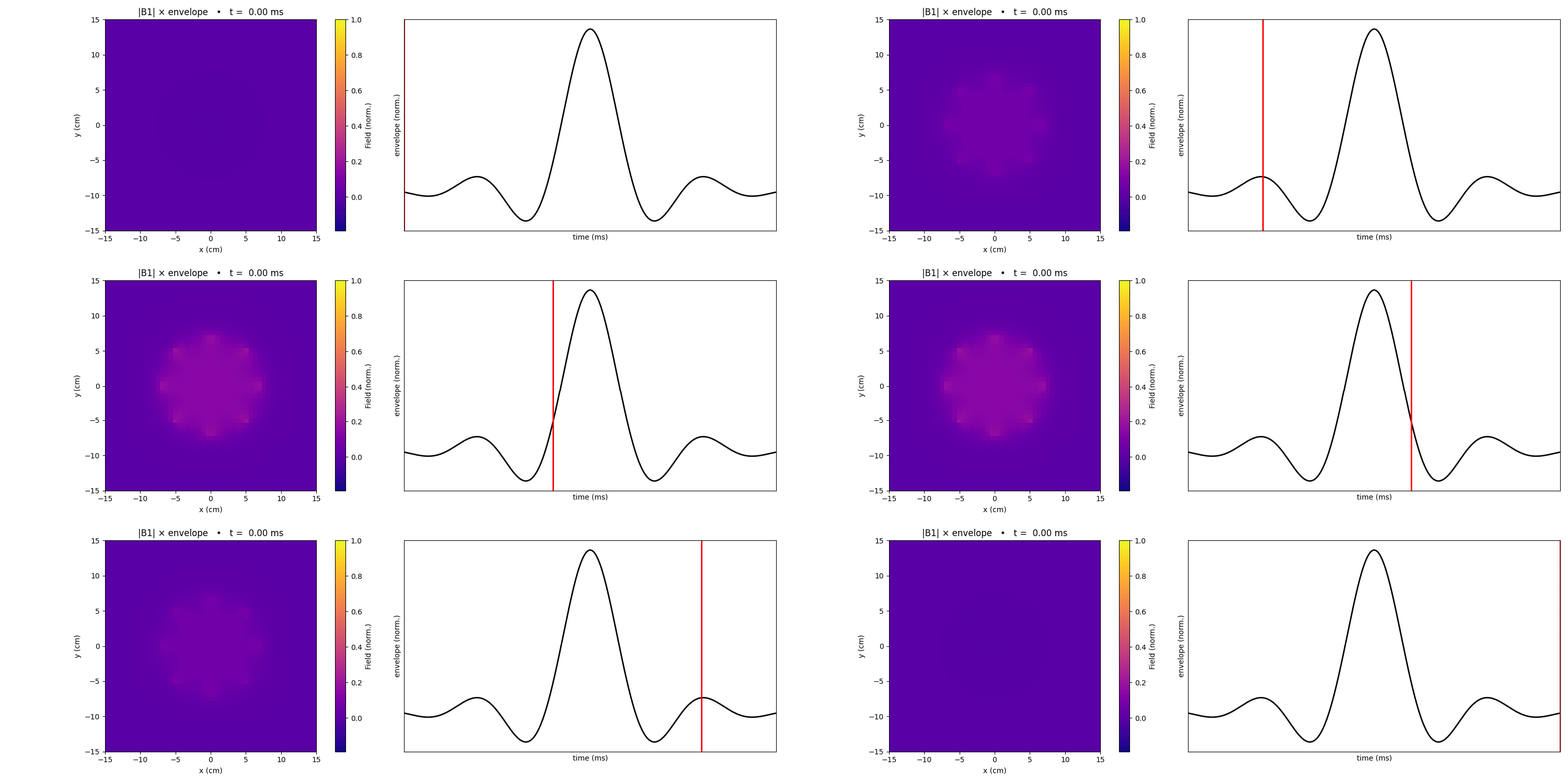
Let's visualize the modulated current in the birdcage with a sinc pulse envelope.
import matplotlib
from matplotlib.colors import Normalize
# animation limit rc parameters
g_norm = pulse.real
matplotlib.rcParams['animation.embed_limit'] = 2**128 # Set a limit for embedded animations
anim_frames = [g_norm[i]*(B1_magnitude) for i in range(Nt)]
anim_frames = np.array(anim_frames) # Convert to numpy array for normalization
anim_frames /= np.max(anim_frames) # Normalize frames for consistent color mapping
# --- Global min/max for fixed normalization ---
global_min = np.min(anim_frames)
global_max = np.max(anim_frames)
norm = Normalize(vmin=global_min, vmax=global_max)
# --- Plot setup ---
fig = plt.figure(figsize=(15,5))
ax_map = fig.add_subplot(1,2,1)
ax_env = fig.add_subplot(1,2,2)
im = ax_map.imshow(anim_frames[0],
extent=(-15,15,-15,15),
cmap='plasma', origin='lower',
norm=norm)
cbar = plt.colorbar(im, ax=ax_map, label='Field (norm.)')
ax_map.set_title('|B1| × envelope')
ax_map.set_xlabel('x (cm)'); ax_map.set_ylabel('y (cm)')
line_env, = ax_env.plot(t*1e3, g_norm, lw=2, color='k')
line_env.set_animated(False) # ← static, baked into the background
vline = ax_env.axvline(t[0] * 1e3, color='r', lw=2)
ax_env.set_xlabel('time (ms)'); ax_env.set_ylabel('envelope (norm.)')
# ax_env.set_ylim(-.1, .1)
ax_env.set_xticks([])
ax_env.set_yticks([]) # Hide y-ticks for cleaner look
ax_env.set_xlim(t[0] * 1e3, t[-1] * 1e3)
ymin, ymax = ax_env.get_ylim()
# --- Animation update ---
def update(i):
im.set_data(anim_frames[i])
vline.set_data([t[i]* 1e3, t[i]* 1e3], [0, 1.05])
ax_map.set_title(f'|B1| × envelope • t = {t[i]:5.2f} ms')
return im, vline
ani = FuncAnimation(fig, update, frames=len(t), interval=10, blit=True)
plt.tight_layout()
plt.close() # Close the figure to avoid displaying it in Jupyter
ani.save("anim3.gif", writer="ffmpeg", fps=30)
pretty_gif("anim3.gif", caption="")
The Resultant Magnetic Field with Sinc Pulse
anim_name = "b1_8_rungs_out_phase_scaled_g_func.gif"
pv_field_animation(
wire_positions,
current_phases,
t, # scale the time to see animation faster
positions,
scaled=True,
g_func=g_norm,
Nt=Nt,
anim_name=anim_name,
)
EmbeddableWidget(value='<iframe srcdoc="<!DOCTYPE html>\n<html>\n <head>\n <meta http-equiv="Content-…
pretty_iframe(f"{anim_name}.html", title="Sinc Modulated Rotating B1 Field")
Sinc Modulated Rotating B1 Field
↳ Source: b1_8_rungs_out_phase_scaled_g_func.gif.html
pretty_gif(anim_name)
@misc{hussain2025rfpulse,
author = {Snawar Hussain},
title = {Simulating RF Pulses and Rotating B₁ Fields in MRI: From Biot–Savart to Quadrature Coils},
year = {2025},
howpublished = {\url{https://snawarhussain.com/simulating-rf-pulses}},
note = {Accessed: 2025-08-26}
}
Copy ⇧⌘C / Ctrl-C
Share on
Twitter Facebook LinkedInComments are configured with provider: facebook, but are disabled in non-production environments.

