
Variational Autoencoders (VAEs) have become increasingly popular in the machine learning field for their ability to perform effective unsupervised learning. They have found a wide range of applications, from image generation to anomaly detection. A key component of VAEs that differentiates them from standard autoencoders is the use of the so-called “reparameterization trick”. This article aims to demystify this concept and provide a clear understanding of its purpose and operation.
What is the Reparameterization Trick?
The reparameterization trick is a mathematical operation used in the training process of VAEs. It’s a technique that helps bypass a significant problem in training VAEs: the backpropagation algorithm cannot be applied directly through random nodes.
The VAE architecture includes a sampling operation where we sample latent variables from a distribution parameterized by the outputs of the encoder. The direct application of backpropagation here is problematic because of the inherent randomness of the sampling operation. In other words, since computing the latent \(z\) involve sampling from a (multivariate normal) distribution. This sampling operation introduce stochasticity and therefore cannot be differentiated.
Note: The reason this operation is stochastic, or random, is because drawing a sample from a probability distribution is a random process. Even though the parameters of the distribution (the mean and variance) are fixed output of the encoder for a given input, the actual samples that you draw from the distribution will vary each time you draw a sample. This is the nature of sampling from a probability distribution
Why Do We Need the Reparameterization Trick?
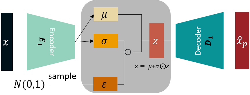
Let’s consider once again the structure of a VAE: it comprises an encoder, a decoder, and a latent space in between. The encoder’s role is to map inputs to a distribution in the latent space, defined by two parameters: a mean \((μ)\) and a standard deviation \((σ)\).
This latent distribution represents the learned representation of the input data. The decoder then generates an output by sampling points from this distribution. However, if we were to sample these points directly, this operation introduces a stochastic element that prevents the direct application of backpropagation.
Backpropagation relies on computing gradients of deterministic (i.e., non-random) operations. Therefore, we need a method that introduces the necessary randomness for sampling while preserving the differentiability of the operations involved. This is where the reparameterization trick comes in.
The backpropagation algorithm, which is used to train neural networks, requires the ability to compute exact gradients. Because the sampling operation is random, it doesn’t have a well-defined gradient (weights always randomly changing). This means that we can’t use the backpropagation algorithm to train the encoder and decoder networks in a VAE.
The Reparameterization Trick Unveiled
The reparameterization trick works by separating the deterministic and the stochastic parts of the sampling operation. Instead of directly sampling from the distribution \(N(μ, σ^2)\), we sample ε from a standard Normal distribution \(N(0, 1)\) and compute the desired sample z as:
\[z = μ + σ * ε\]Here, \(ε\) introduces the necessary randomness. The operation \(μ + σ * ε\) is entirely deterministic and differentiable, meaning we can apply backpropagation through it.
This method allows us to incorporate the random element required for sampling from the latent distribution while preserving the chain of differentiable operations needed for backpropagation.
Why Not \(μ + σ\)?
You might be wondering why we can’t simply compute \(z\) as \(μ + σ\). Without the randomness introduced by \(ε\), every time we run the encoder with the same input, we’d get the exact same output \(z\). This does not reflect the probabilistic nature of the latent space that we’re trying to model.
In addition, during training, we want the model to learn to map an input to a region in the latent space, not just to a single point. This is made possible by the randomness introduced by \(ε\), which is key to the model’s ability to generate diverse outputs during the decoding process.
Conclusion
The reparameterization trick is a powerful method that makes the training of VAEs possible and efficient. By cleverly separating the random and deterministic elements of the sampling operation in the VAE, it allows us to leverage the power of backpropagation while maintaining the stochastic nature of the model. Understanding this trick is key to gaining a deeper insight into the workings of VAEs and their various applications in machine learning.
Share on
Twitter Facebook LinkedInComments are configured with provider: facebook, but are disabled in non-production environments.