
Photometric Stereo
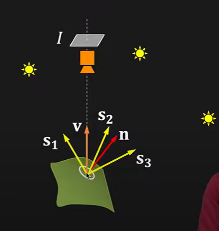
Given the intensity of one pixel in an image does not provide information about the surface orientation or surface normal \(n\) of the object at that particular point. Photometric stereo uses multiple images of an object taken under different light conditions from different angles to get the surface orientation. The images of an object taken under different light conditions \(S\) gives us the measure of multiple intensities values of each pixel under these lighting conditions. Given that We have measured the image intensity values \(i\) produced by each of the light source \(S_i\) These intensities values help resolve the ambiguity to estimate the surface orientation. In simpler words, Photometric stereo is a way to estimate the 3D shape of an object from images of the same object taken with different light sources oriented at different positions.
Assumptions:
- The camera viewing angle \(V\) is same for all points on the surface
- For each individual light source \(S\) the direction is same for all points on the surface.
in other words, the camera is far away and the light sources are far away.
Basic Idea
Step 1: Acquire \(K\) images with \(K\) known light sources
Step 2: Using known source direction and \(BRDF\), construct reflectance map for each source direction.
Step 3: For each pixel location \((x, y)\), find \((p, q)\) as the intersection of \(K\) reflectance curves from different light sources. This \((p, q)\) gives the surface normal at pixel \((x, y)\)
The smallest \(K\) values depends on the surface properties of a material.
Lambertian surface case
For a lambertian surface three light sources ( \(K = 3)\) is enough to compute the surface normals \(n\) and the albedo. The assumption for a lambertian surface is that light from each source can reach each point on the surface.
Photometric stereo: Lambertian Case
For doing photometric stereo with the lambertian model of the diffused reflections we model the equation so such that: Image intensities measure at a point \((x, y)\) of the object or at the pixel of the image under three different light sources is given as:
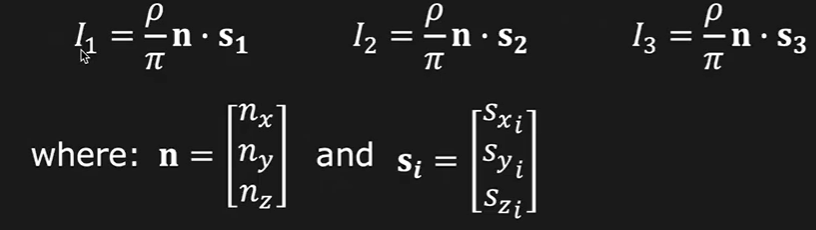
Where \(I_i\) is the image intensity for each light source \(s_i\). Here \(n\) is the unit normal vector that is normal to the surface or in this case, normal to the particular pixel in the image. \(\rho\) is the albedo of the image. the \(\pi\) can be ignored for the simplicity
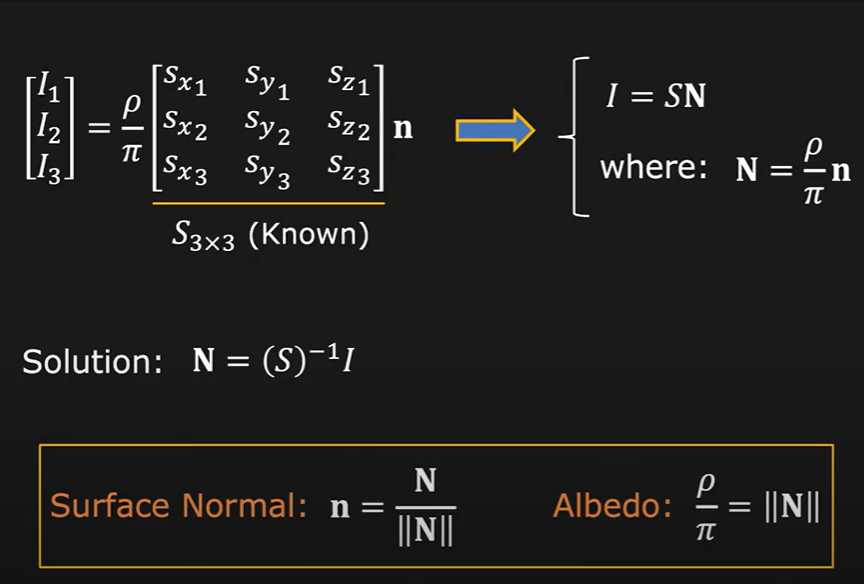
The above three equations can be expressed as in matrix form as shown in below:
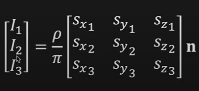
The image intensities values are given as a vector \([I_1 ... I_3]\) that we had measured on each point in the image. and the \(S\) is a known \(3*3\) matrix for three different light sources that are known to us. from this set of equation the we have 2 unknowns that are the image albedo and the surface normal vector \(n\) We speculate that the image albedo is not constant rather vary from point to point.
Given these measurements and set of assumptions we can solve the matrix equation for \(n\) and the albedo the solution is given below:
Code Implementation
Understanding the data
The given data consists of individual objects (bear, buddha, cat, and pot) that are captured under 96 unique light sources. the object under each light source corresponds to a 16 bit RGB image. The light source directions for each source are given in ‘light_directions.txt’. After loading, Images are normalized by dividing each channel to their corresponding intensity value given in ‘light_intensities.txt’. each object comes with a binary mask as well.
Loading dataset and normalizing it with the intensity values
import random

import cv2
import glob
import re
import os
import numpy as np

def numerical_sort(value):
    numbers = re.compile(r'(\d+)')
    parts = numbers.split(value)
    parts[1::2] = map(int, parts[1::2])
    return parts

def imread(file_name, intensities=None, flag=-1, scale=1.0):
    img_names = glob.glob(file_name)
    img_list = []
    if len(img_names) == 0:
        print("[No {} images]".format(file_name))
        exit()
    img_names = sorted(img_names, key=numerical_sort)
    for i, path in enumerate(img_names):
        img = cv2.resize(cv2.imread(path, flag), None, fx=scale, fy=scale)
        if  np.any(intensities):
            img = img / intensities[i]
        img_list.append(img)
    return img_list
from numpy import loadtxt

dataPath = "data/"
object = []
for obj  in (os.listdir(dataPath)):
    object.append(obj)

L_direction = loadtxt(f"data/{object[0]}/info/light_directions.txt")
intensities = loadtxt(f"data/{object[0]}/info/light_intensities.txt")
path_img = "data/bearPNG"

imgs = imread(path_img + f"/{object[0]}/*", intensities=intensities)
mask = imread(f"data/{object[0]}/info/mask.png")[0]
Applying the mask to the image
Applying the mask to the images, makes anything outside the boundry of our object of interest zero. this makes the subsequent computations a bit faster as well as allows us to only compute surface normals of the object and not for the background in the image.
for i, bear in enumerate(imgs):
    imgs[i] = cv2.bitwise_and(bear, bear, mask=mask)
    i += 1

imgs = np.array(imgs)
Photometric Stereo code implementation
Given the masked images and the light source direction \(S_i\) corresponding to each image. We can calculate the photometric stereo in lambertian model using the equations described in Section 2 above.
Since these given equations are for computing surface normals and albedo for a given point or pixel in the image. The acutal coding implementation is much more complex since we have an RGB 16 bit image that has 3 channels R, G and B with each channel having 512 x 612 pixels. this makes the computation much harder. since we have to loop through the given 3 RGB images pixel by pixel . Since we require at least 3 images to compute the surface normal for a given pixel.
For given images the intensities
After solving the matrix equation for each pixel in the set of 3 images we get our albedo and surface normal matrix \(n\) for each pixel.
The (x y z) coordinate of the surface normal need to be converted to RGB coordinates for that we use
def PMS(imgs, L_list):
    """
    This is the main function for performing photometric stereo using three images.

        Parameters
        ----------
        imgs: np.ndarray
            ndarray of all the images of an object taken with different light sources
        L_list: list
            the list of the light sources directions S for each image. for each image the S is a vector matrix with 3  positional elements (x,y,z)
        return:
            returns the computed albedos and the surface normals of the object
    """


    L = np.array(L_list)
    Lt = L.T
    h, w = imgs[0].shape[:2]

    img_normal = np.zeros((h, w, 3))
    img_albedo = np.zeros((h, w, 3))
    I = np.zeros((len(L_list), 3))
    for x in range(w):
        for y in range(h):
            for i in range(len(imgs)):
                I[i] = imgs[i][y][x]                           #getting intensities for the 3 images to construct the Intensity vecotr

            tmp1 = np.linalg.inv(Lt)

            N = np.dot(tmp1, I).T
            rho = np.linalg.norm(N, axis=1)
            img_albedo[y][x] = rho

            N_gray = N[0]*0.0722+N[1]*0.7152+N[2]*0.2126  #luminosity formula
            Nnorm = np.linalg.norm(N)
            if Nnorm==0:
                continue
            img_normal[y][x] = N_gray/Nnorm

    img_normal_rgb = ((img_normal*0.5 + 0.5)*255).astype(np.uint8)  #(x y z) cooridinate to RGB coordinate converstion.
    img_normal_rgb = cv2.cvtColor(img_normal_rgb, cv2.COLOR_BGR2RGB)  #converting from BGR to RGB for correct visualization. cv2 uses BGR format.
    img_albedo = (img_albedo/np.max(img_albedo)*255).astype(np.uint8)
    return img_normal, img_albedo, img_normal_rgb
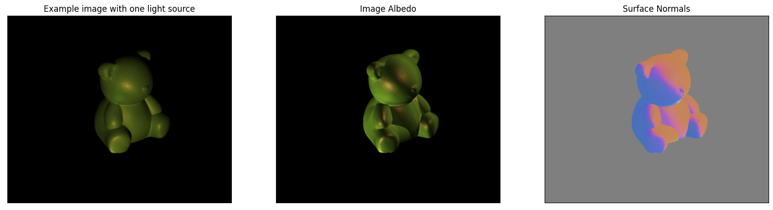
Sample 3 images randomly from data for constructing surface normals and albedo
import matplotlib.pyplot as plt
import random
random.seed(5)
index = random.sample(range(0,96), 3)
img_normal, img_albedo, img_normal_rgb = PMS(imgs[list(index),:], L_direction[list(index),:])
Plotting…
plt.figure(figsize=(20,5))
plt.subplot(1,3,1)
#
img = (imgs[1] - np.min(imgs[1])) / (np.max(imgs[1]) - np.min(imgs[1]))  #normalizing image between 0-1 for visualization
plt.imshow(img)
plt.title('Example image with one light source')
plt.xticks([])
plt.yticks([])
#plt.plot([1,2,3,4])
plt.subplot(1,3,2)
#plt.plot([1,2,3,4])
plt.imshow(img_albedo)
plt.title('Image Albedo')
plt.xticks([])
plt.yticks([])
plt.subplot(1,3,3)
#plt.plot([1,2,3,4])
plt.imshow(img_normal_rgb)
plt.title('Surface Normals')
plt.xticks([])
plt.yticks([])
plt.show()
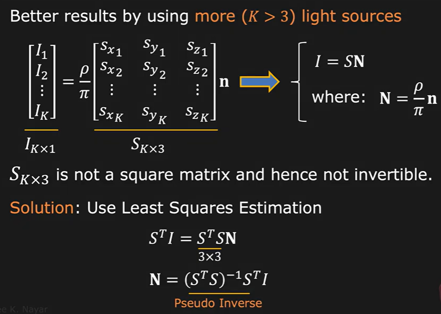
4. Using more than 3 images
what if we can use more than 3 images or all the available images for photometric stereo?
Probelm: The matrix \(N\) becomes non-square and non-invertable so it’s inverser can not be found.
Solution: Use pusedo inverse of matrix \(N\) where we multiply both side of the equation given in section 2 with the transpose of the \(N\) matrix
def PMS_all(imgss, L_list):
    """
    This is the main function for performing photometric stereo using three images.

        Parameters
        ----------
        imgs: np.ndarray
            ndarray of all the images of an object taken with different light sources
        L_list: list
            the list of the light sources directions S for each image. for each image the S is a vector matrix with 3  positional elements (x,y,z)
        return:
            returns the computed albedos and the surface normals of the object
    """


    L = np.array(L_list)
    Lt = L.T
    h, w = imgss[0].shape[:2]

    img_normal = np.zeros((h, w, 3))
    img_albedo = np.zeros((h, w, 3))
    I = np.zeros((len(L_list), 3))
    for x in range(w):
        for y in range(h):
            for i in range(len(imgss)):
                I[i] = imgss[i][y][x]


            tmp1 = np.linalg.inv(np.dot(Lt, L))   #inverse of L
            tmp2 = np.dot(Lt, I)       # L_inv * I

            N = np.dot(tmp1, tmp2).T
            rho = np.linalg.norm(N, axis=1)
            img_albedo[y][x] = rho

            N_gray = N[0]*0.0722+N[1]*0.7152+N[2]*0.2126  #luminosity formula for converting datato RGB colorspace.
            Nnorm = np.linalg.norm(N)
            if Nnorm==0:
                continue
            img_normal[y][x] = N_gray/Nnorm

    img_normal_rgb = ((img_normal*0.5 + 0.5)*255).astype(np.uint8)  #converting the 16 bit data to 8bit ranging from 0-255 for visualization
    img_normal_rgb = cv2.cvtColor(img_normal_rgb, cv2.COLOR_BGR2RGB)  #converting from BGR to RGB for correct visualization. cv2 uses BGR format.
    img_albedo = (img_albedo/np.max(img_albedo)*255).astype(np.uint8)
    return img_normal, img_albedo, img_normal_rgb
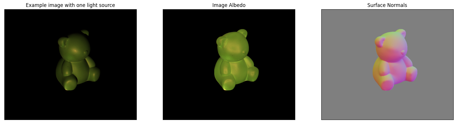
img_normal, img_albedo, img_normal_rgb = PMS_all(imgs, L_direction)
Results are improved after using more images
plt.figure(figsize=(20,5))
plt.subplot(1,3,1)
#
img = (imgs[1] - np.min(imgs[1])) / (np.max(imgs[1]) - np.min(imgs[1]))  #normalizing image between 0-1 for visualization
plt.imshow(img)
plt.title('Example image with one light source')
plt.xticks([])
plt.yticks([])
#plt.plot([1,2,3,4])
plt.subplot(1,3,2)
#plt.plot([1,2,3,4])
plt.imshow(img_albedo)
plt.title('Image Albedo')
plt.xticks([])
plt.yticks([])
plt.subplot(1,3,3)
#plt.plot([1,2,3,4])
plt.imshow(img_normal_rgb)
plt.title('Surface Normals')
plt.xticks([])
plt.yticks([])
plt.show()
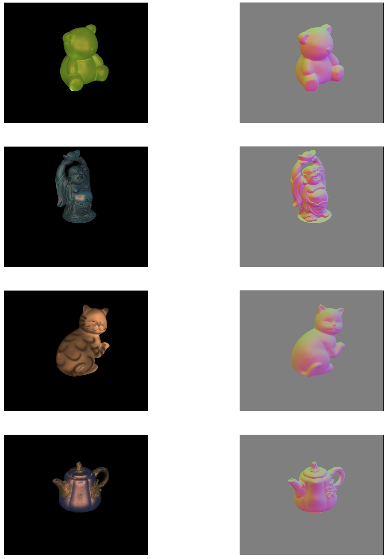
Similarly results for the rest of the objects
The Photometric stereo is iteratively applied to each of the object. The code loads data related to each object, estimate the photometric stereo paramerters (albedo, surface normal) and appends them to a list. The results saved in the list are then can be unrolled and visualized and can be used for post-hoc analysis.
import os
dataPath = "data/"
object = []
for obj  in (os.listdir(dataPath)):
    object.append(obj)
imgs = []
mask = []
L_direction =[]
intensities = []
results = []

for i, ob in enumerate(object):
    L_direction.append(loadtxt(f"data/{ob}/info/light_directions.txt"))
    intensities.append(loadtxt(f"data/{ob}/info/light_intensities.txt"))
    path_img = f"data/{ob}"
    imgs.append(imread(path_img + f"/{ob}/*", intensities=intensities[i]))
    mask.append(imread(f"data/{ob}/info/mask.png")[0])
    for j, object in enumerate(imgs[i]):
        imgs[i][j] = cv2.bitwise_and(object, object, mask=mask[i])

    imgs[i] = np.array(imgs[i])

    results.append(PMS_all(imgs[i], L_direction[i]))
import matplotlib.pyplot as plt
plt.figure(figsize=(30,25))
for i in np.arange(0,4):
    # plt.subplot(4,3, i+1)
    # plt.imshow(imgs[i][0])
    # plt.xticks([])
    # plt.yticks([])
    for j in np.arange(1,4):
        loop = j+(i*3)
        if loop in [1, 4,7,10]:
            continue
        else:
            plt.subplot(4,3, loop)
            plt.imshow(results[i][j-1])
            plt.xticks([])
            plt.yticks([])
4. Conclusion
In this tutorial,
-
First, the concept of photometric was briefly described. It was demonstrated that under the constraints of certain assumptions, the equations for the photometric stereo for a lambertian reflectance model can be easily derived. These equations can be solved for estimating the surface normals and the albedo at each point of an object given its \(K\) set of images under different lighting conditions.
-
Algorithm for the photometric stereo was then implemented and the output results were shown after performing various transforms (namely: luminosity weighting, RGB color space conversion, RGB to BGR conversion etc.) to make the output suitable for visualization.
-
Then the photometric stereo was modified to include more than 3 images.Taking advantage of the fact that we have 96 images of each object taken under different light conditions. The resultant albedo and surface normal map looks much better than the ones estimated using 3 images.
Give the surface normals, next thing that can be done is heightMap or depth estimation and 3D re-randering of the object.
Share on
Twitter Facebook LinkedInComments are configured with provider: facebook, but are disabled in non-production environments.