Image Stitching: Combining multiple images of an overlapping scene

Image Stitching

Image stitching is a classis computer vision problem where given the multiple images of a scene taken from a same view point but with slightly different panning (rotating the camera). Given that few regions in the images overlap, we are required to synthesize an image (panorama) that is combination of all the given images and provides the whole scene covered by them.

The process of image stitching involves following steps.

1. Recognizing different features of the images using algorithms like SIFT.
2. Calculating descriptors for the detected features.
3. Matching corresponding features across multiple images.
4. Applying RANSAC to detect the outliers or false positive matches.
5. Computing Homography using the inliers or true positive matches.
6. Transforming the source image(s) using the homography matrix
7. Fusing source image(s) with the destination image and performing Image blending

This reports contains the observations and understanding of the above steps made while implementing the image stitching code

Feature Detection and Description

For feature detection and description we can use the SIFT feature detector and descriptor. python opencv package has pre-implemented this. First we use SIFT algorithm to detect various important and distinct regions of interest in the image as features.

Along with normalized detected features, SIFT also returns a computed description of each of the feature/keypoint as a 128 dimensional vector.

Once we have the features and their description, the next step is to match these features across.

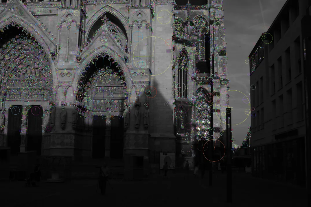
Fig1: Detected sift features drawn on the image

Feature Matching

Feature matching refers to recognize the correspondence between features of two different images with overlapping regions of a scene. Feature matching is a one-to-one correspondence. Given two images of a scene. SIFT can recognize up to 1000+ features and their description for each single image. Having features of such great magnitude, to find a one to one correspondence between these features is computationally an expensive task.

One naive implementation would be to take each feature descriptor from the source image and calculate L2 norm of all the descriptors in the destination image for that specific source descriptor. The descriptor with the lowest L2 norm in the destination image indicates greater similarity with the source features. This way of feature matching is usually called “Brute Force matching”.

In this code, Brute Force matching was implemented. Since python is an interpreted language therefore, the run time of this algorithm is very long given we have 10000+ features in each image. The code implementation is given below:

def matchFeatures01(kp1, kp2, des1, des2, img1, img2):
    matches = {'queryIndx': [],
               'trainIndx': []
               }
    np.random.seed(2)
    idx2 = np.random.choice(np.arange(0, len(des2)), 7000, )
    idx1 = np.random.choice(np.arange(0, len(des1)), 7000, )
    des2 = des2[idx2]
    for i, des in enumerate(des1[idx1]):
        dists = np.linalg.norm((des - des2), axis=1) ** 2
        sorted_dist = np.sort(dists, axis=0)
        if sorted_dist[0] < 0.75 * sorted_dist[1]:
            matches['queryIndx'].append(idx1[i])
            matches['trainIndx'].append(idx2[np.argsort(dists)][0])
        else:
            continue
    return matches

For each source feature, two closest features in the destination image are considered. Because in many cases, the second closest-match may be very near to the first. It may happen due to noise or some other reasons. In that case, ratio of closest-distance to second-closest distance is taken. If it is greater than 0.75, they are rejected. This can eliminate around 90% of false matches (source: opencv-website)

RANSAC Algorithm for Computing Homography

Once the feature matching is done and correspondence between source to destination features is made. Next step is to apply RANSAC algorithm to compute homography matrix.

Pitfalls:

Although RANSAC algorithm may seem straightforward, there are several pitfalls when it comes to implementing it from scratch in the context of computing homography matrix.

First of all, there is a confusion related to the choice of model for detecting inliers and outliers. In the context of machine learning, RANSAC is commonly used for curve fitting like Linear Regression where we are given with input samples \(x\) and some labels \(y\). However, for homography we don’t have these so called labels and not everything is laid out.Step by step RANSAC algorithm implementation for homography is given as followed:

From feature matching output, randomly select 4 of the correspondence. Correspondence is given as feature points from source image \([x_s y_s 1]\) and destination image \([x_d y_d 1]\) . We get 8 of these points from 4 randomly select matching pairs or correspondences.

1. Give these 8 points construct the 8 x 9 \(A\) matrix and compute the eigen vectors using svd decomposition.
2. Compute the Homography matrix \(H\) as the last eigen vector and reshape it into a 3x3 matrix of \(H\)
3. Once homography is computed, transform all the key points of source using homography and compute the geometric distance (error) between the estimated transformed of source and the actual keypoint in the destination image.
4. source keypoints with error below a threshold are inliers while the rest are outliers.
5. Keep Repeating the process from step 1 until the total number of inliers reach a certain threshold.

Corr size:  5851  NumInliers:  5 Max inliers:  15
Corr size:  5851  NumInliers:  747 Max inliers:  747
Corr size:  5851  NumInliers:  1066 Max inliers:  1066
Corr size:  5851  NumInliers:  9 Max inliers:  1066
Corr size:  5851  NumInliers:  2729 Max inliers:  2729
Corr size:  5851  NumInliers:  11 Max inliers:  2729
Corr size:  5851  NumInliers:  1180 Max inliers:  2729
Corr size:  5851  NumInliers:  4120 Max inliers:  4120

Caption: RANSAC algorithm in action.

Once RANSAC has done it’s job. Compute the homography matrix again with all inliers found using RANSAC instead of just using 4 matching pairs.

Image transforming and Stitching

The final computed homography matrix \(H\) can now be used to tranform the whole image using a pixel by pixel transform.

Next step is to merge the transformed source image and the destination image. Which may seem easier but turns out to be quite complicated.

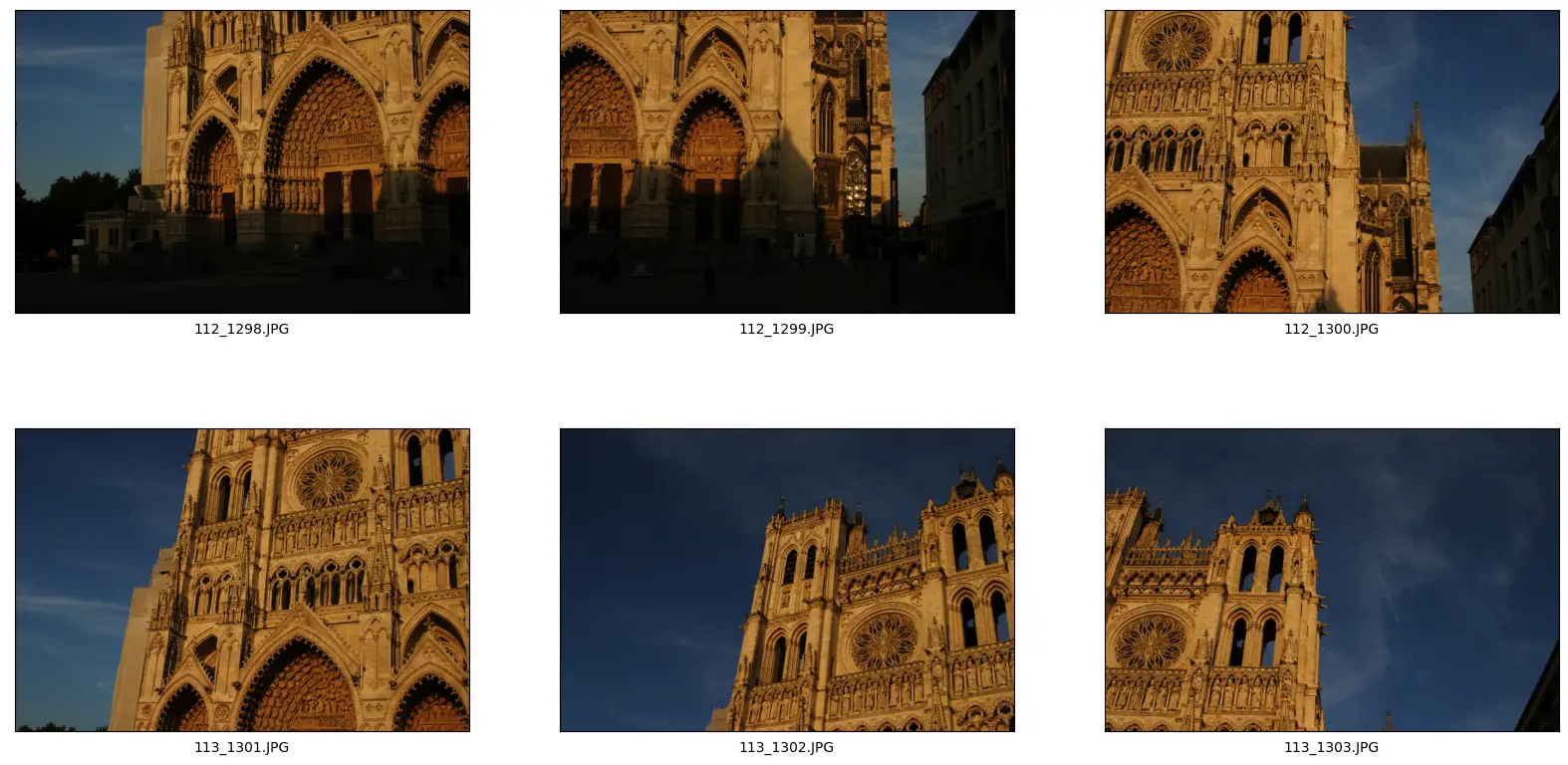
In this code implementation. First the source image was transformed and empty region was added to either left or right depending on the relative direction of it from the destination image. Source and destination images were chosen arbitrarily and the according to the most convenient format. For example in the Fig2, after looking at the image it can be noticed that image 112_1299.JPG can be transformed and stitched with 112_1298.JPG in the left direction.

Additionally it is required to adopt different strategies for stitching the images in horizontal and vertical direction. For that an argument orient is passed to the function main() to determine the orientation.

Horizonal Stitching

Based on intuition, first the images that can be horizontally stitched are stitched together. As shown in Fig 03

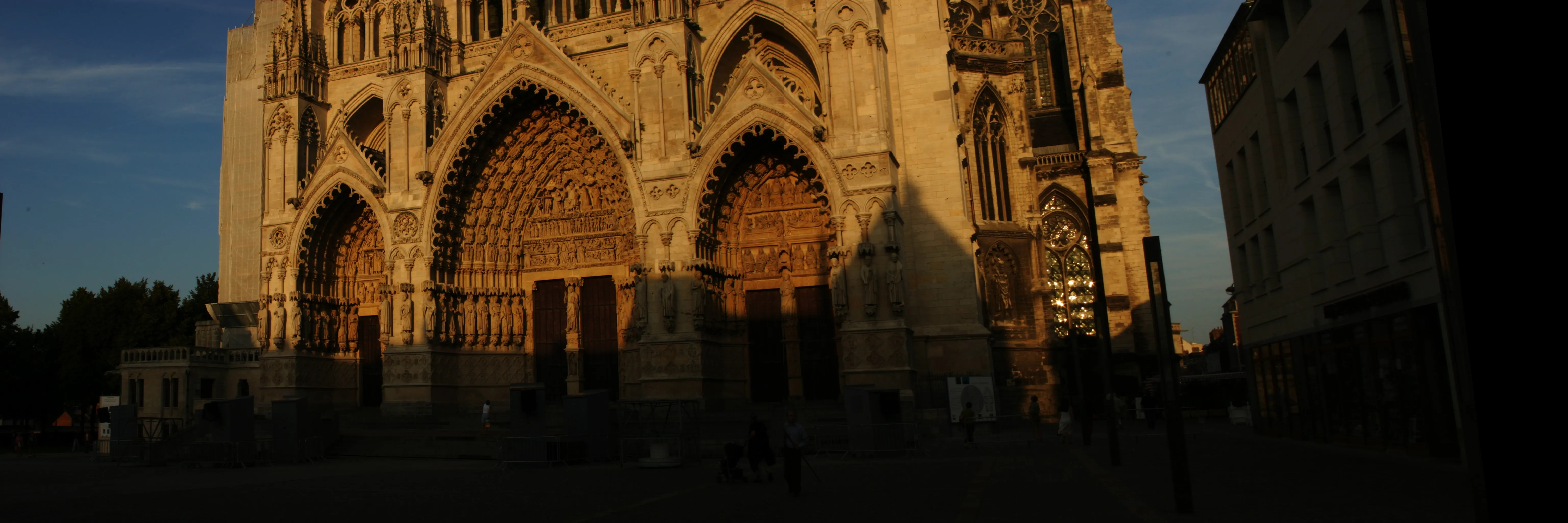
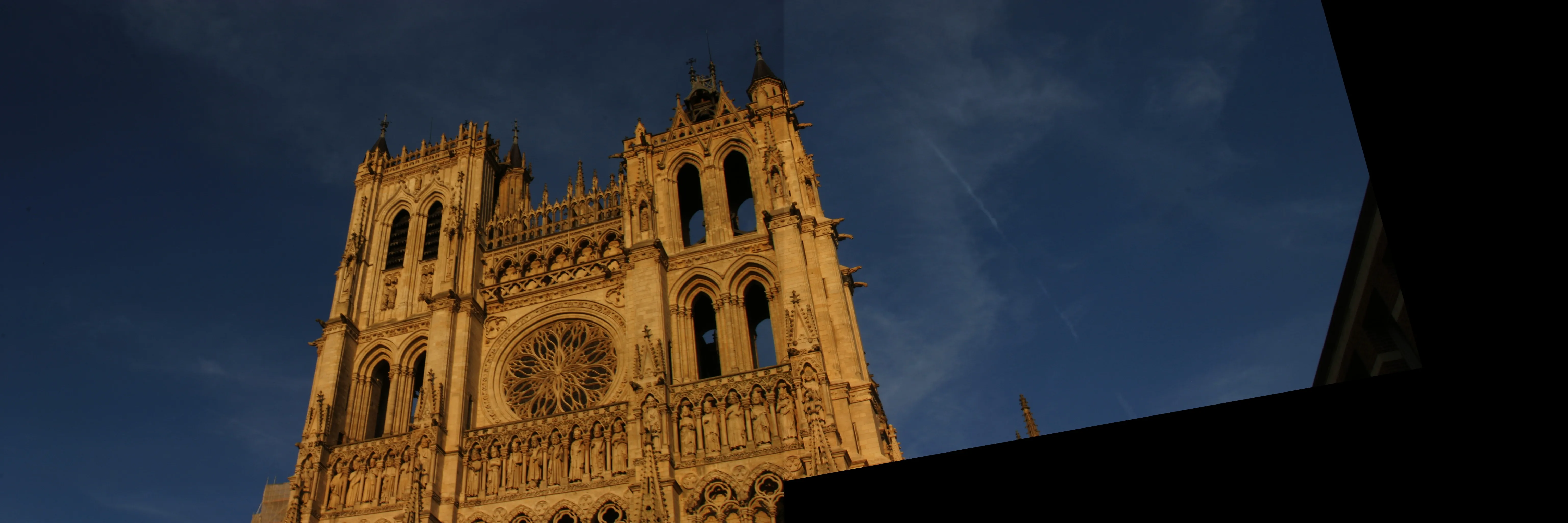
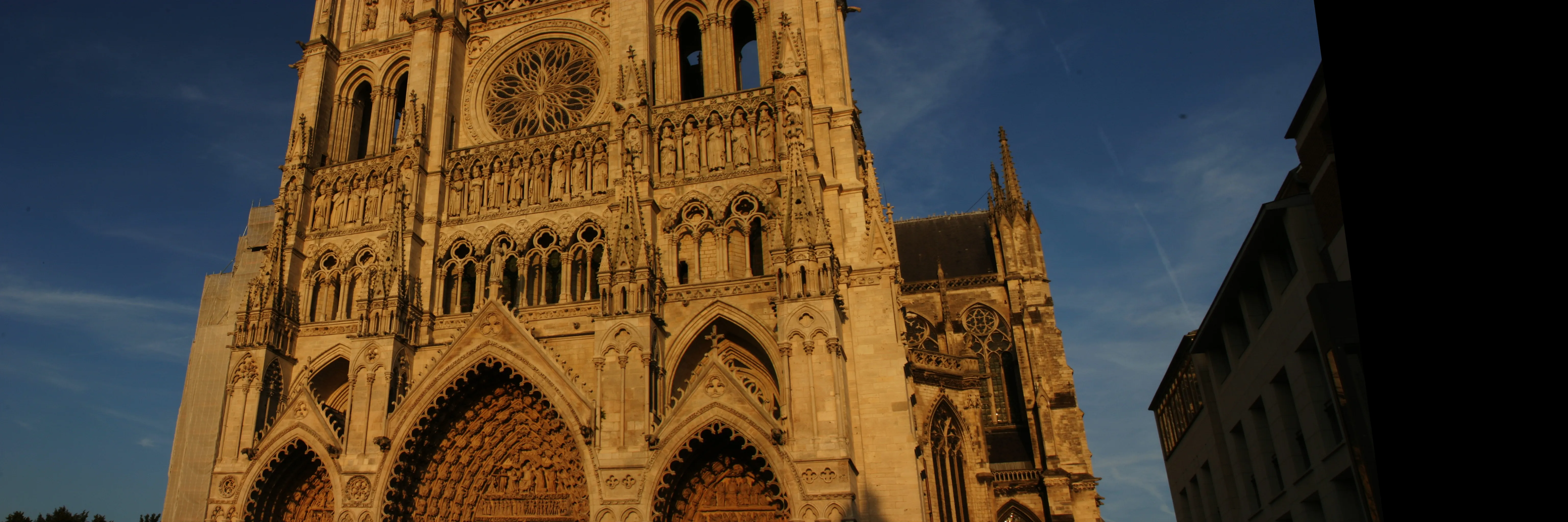
Fig 03: Horizontally stitched images

Vertical Stitching

Horizontally stitched images are then again taken and stitched vertically to form the complete image of the church. for the choice of blending, the simple pixel replacement was used in horizontal stitching and it proves to be quite effective given that the images don’t have high difference in exposer. For vertical stitching the pixel replacement this strategy ends up poorly performing as empty regions of the source image might replace/hide some regions in the destination image since there are no masks to be used. For vertical stitching , bitwise logical operations can reveal the overlapped regions better but the color integrity is gone as shown in Fig04 (a). The other options is to weighted addition of images using opencv built-in function addWeighted() Fig04 (b). Both of them don’t quite work well. However image blending might be a complete assignment in itself so any advance blending options were left out for convenience and simplicity.

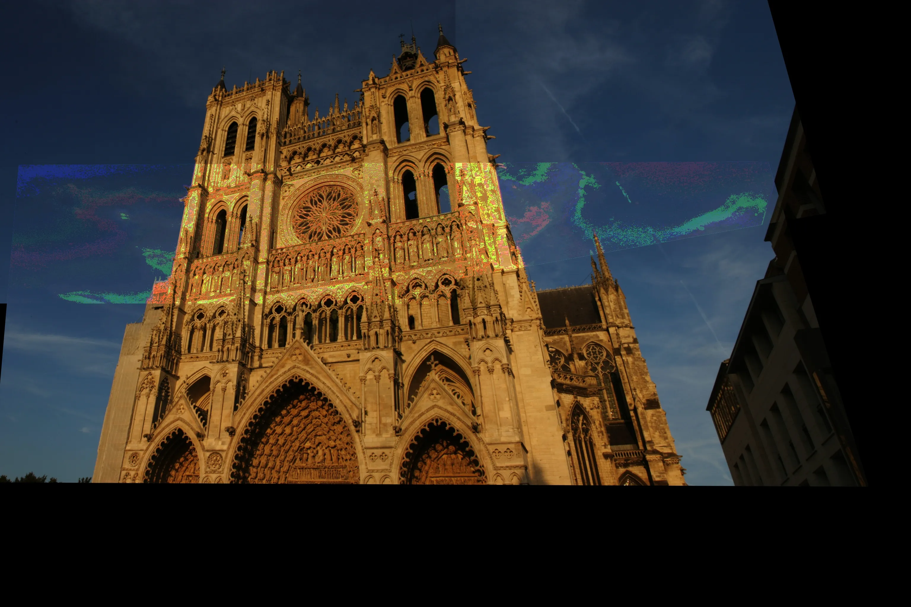
Fig04 (a): Vertical stitching with bitwise OR operation blending

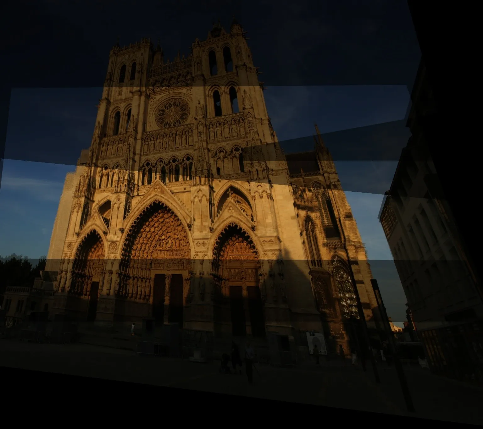
Fig04 (b): Final vertical stitching with weighted blending

dst[0:img2.shape[0], 0:img1.shape[1]] = img1_color

Code Caption pixel replacement blending/merging

Closing Remarks

• It was particularly difficult to figure out the right blending option and implement orientation based stitching.
• Many concept related to RANSAC for computing homography are not made clear so it can be challenging to determine the right steps to achieve it.
• Feature matching though was easier, but it’s vectorized and more optimized version could not be implemented and the current version of brute force matching is painfully slow.
• Due to the long running time of feature matching, only a portion of SIFT descriptors are considered (7000 to be precise) this means that many important descriptors might be missed. and the errors from matching are carried forward to the end results.
• The Full code for image stitching from scratch can be found on my Github