
Introduction
In Magnetic Resonance Imaging (MRI), gradient fields, among many other things, are used to encode spatial information. This post aims to clarify the connection between gradient fields and spatial frequencies in the K-space, and how gradients walks us through K-space. Blending mathematical theory with practical code examples, the goal is to enhance basic understanding of MR Physics and Simulation.
Mathematical relationship between K-space and Gradient fields
Recall from MRI theory that the gradients are used to change the mangetic field strenght of the B0 field in a particular direction. For example a gradient in the x direction will change the magnetic field strength in the x direction.And similar is the case with gradients in the y or z direction.This change in magnetic field strength is represented by the following equation:
\[B(x,y,z) = (B_0 + G_x.x + G_z.y+ G_z.z)_z\]It is important to note that the overall magnetic field is still pointing in the z direction. The gradients only change the strenght of magnetic field in space and not the direction. That is why the right side of the above equation is subscripted with z. visually we can represent this change in magnetic field strength as shown in the following interactive plot: by changing slider values we can change the magnetic field strength in the x, y and z directions. the overall magnetic field is still pointing in the z direction. The gradients only change the strenght of magnetic field shown in colorcoded arrows all pointing in the z direction.
Rotating vs Labratory Frame of reference
Consider a simple scenario where follwing an RF field and a slice selection gradient, we have a 2D slice of the spin magnetic moments knocked into the transverse plane all rotating at larmor frequency in phase.
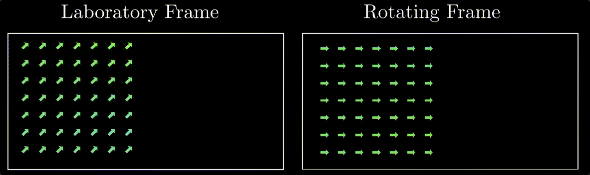
In the laboratory frame of reference, the spin magnetic moments are precessing at the Larmor frequency and are initially in phase. However, when we shift our perspective to the rotating frame of reference, these spin magnetic moments appear stationary. This stationary appearance results from the rotating frame moving synchronously with the spins’ Larmor precession. This concept is at the core of what we call the rotating frame of reference.
Opting for the rotating frame of reference in our subsequent discussions offers a significant advantage. It simplifies the visualization of gradient effects on spin magnetic moments, allowing us to observe these effects without the complexity introduced by their rapid precession in the laboratory frame. Essentially, it provides a clearer and more stable viewpoint, making it easier to comprehend the changes induced by the gradients without the ‘dizzying’ effects of spin motion seen in the lab frame.
Gradient Fields and Spin Magnetic Moments
When a gradient field is introduced in any direction, it alters the magnetic field strength along that direction. This variation in magnetic field strength causes the spin magnetic moments to precess at different frequencies in that specific direction. The reason for this is that the precession frequency of spin magnetic moments is directly proportional to the magnetic field strength, as described by the equation:
\[\omega = \gamma B\]Here, \(\omega\) represents the precession frequency, \(\gamma\) is the gyromagnetic ratio, and \(B\) signifies the magnetic field strength.
In a rotating frame of reference, this differential in precession frequencies translates to spin dephasing along the spatial gradient. This dephasing occurs because spins are not precessing synchronously with the rotating frame.
For instance, a Gx gradient introduces spin magnetic moment dephasing along the x-axis. Spins located on one side of the x-axis origin dephase in the opposite direction to those on the other side, while spins precisely at the x-axis origin do not dephase. Analogous effects occur with Gy and Gz gradients, affecting spin dephasing along the y-axis and z-axis, respectively.
2D Fourier Transform and MRI
In our previous discussion on 2D Fourier Transform we simplified the concept of image decomposition using the principles of the 2D Fourier Transform. To avoid the complexities of mathematical rigor, let’s recall the key idea: any two-dimensional (2D) spatial signal, such as an image, can be decomposed into components resembling 2D sinusoids. These sinusoidal patterns represent variations in both spatial frequency and phase orientation. By gathering enough amount of these 2D sinusoids, varying in their spatial frequencies and orientations, we can reconstruct the original image. This process forms the crux of the inverse 2D Fourier Transform.
Each of these 2D sinusoids, characterized by specific oscillations along the x and y axes, correlates to a unique point in the 2D Fourier Transform plane, denoted as \(F(k_x, k_y)\). This plane is, in fact, what is known in MRI terminology as the K-space. K-space is a conceptual framework used for understanding and processing the data acquired by MRI scanners to produce images. It represents the spatial frequencies of the object being imaged, with each point in K-space contributing to the overall image’s formation.
Stepping Through K-space using Gradients
The role of gradients in MRI is pivotal for navigating through K-space, and to demonstrate this, I have created an interactive graph. Imagine a 2D slice with spin magnetic moments initially aligned in the transverse plane and rotating at the Larmor frequency, in phase within the rotating frame of reference.
In our interactive plot, you’ll find horizontal and vertical sliders representing the application of gradient fields. As you adjust these sliders, you are effectively changing the frequency and phase of the spin magnetic moments. This adjustment simulates the effects of frequency and phase encoding in MRI.
The horizontal slider corresponds to the frequency encoding gradient. Moving this slider alters the precession frequency of the spins along one axis, thus varying their position along the frequency-encoded direction in K-space.
The vertical slider, on the other hand, represents the phase encoding gradient. Adjusting this slider changes the phase of the spins, thereby moving them along the phase-encoded direction in K-space.
As you interact with these sliders, observe the changes in a 2D grid of arrows on the plot. These arrows symbolize the spin magnetic moments and their orientation in response to the applied gradients. Were you able to see it ??
By turing on the gradients in the x and y direction we are varying the frequency and phase of the spins in the x and y direction based on their location in space and in-turn creating our own 2D sinosoids corresponding to a certain point in the 2D K-space.
This is exactly what we do in MRI. We collect 2D sinosoids (of spin magnetic moments of different tissues) varying in spatial frequency and phase and once we have collected enough of them we can reconstruct the original image back using the inverse Fourier Transform.
Mathematically, the relationship between the gradient fields and their representation in K-space can be expressed as follows:
\[k(x,y,z) = \gamma \int G(x,y,z) dt\]In this equation, \(k(x,y,z)\) represents the position in K-space , \(\gamma\) is the gyromagnetic ratio, \(G(x,y,z)\) is the gradient applied, and \(dt\) denotes the integration over time. This formulation illustrates that the position in K-space is directly proportional to the time integral of the gradient field applied in a arbitrary direction.
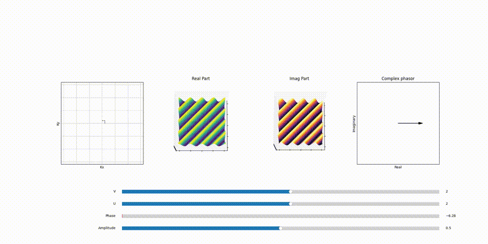
The Influence of \(k_x\) and \(k_y\) on Sinusoidal Patterns
Recall that the number of wiggles or oscillations in 2D sinosoid in x and y direction correlates directly to a specific point in the \(F(k_x, k_y)\) plane aka K-space. For instance, a sinusoid with 3 complete cycles in the x-direction and 3 in the y-direction would correspond to a point in \(F(k_x, k_y)\) with \(k_x =3\) value and \(k_y =3\) value. This mapping is fundamental to how spatial frequencies are represented and manipulated in the Fourier Transform, particularly in applications like MRI, where precise spatial information is crucial.
Here’s a part of animation that demonstrates the relation between point in K-Space and the 2D sinosoid it generates and the effect of phasor assosiated with each of the 2D sinosoid (spatical frequency) and how it scales and shifts it.
Conclusion
In summary, the intricacies of MRI technology, particularly the role of gradient fields in navigating through K-space, underscore the sophistication of this imaging modality. Through the careful manipulation of gradients, MRI is capable of encoding spatial information into the spin magnetic moments, which are then mapped onto K-space. The fundamental equation \(k = \gamma \int G dt\) elegantly captures this relationship, demonstrating how the position in K-space is determined by the integrated effect of the applied gradients over time.
This deep interplay between physical principles and technological implementation not only facilitates the creation of detailed anatomical images but also opens avenues for advanced imaging techniques. The interactive tools and visualizations we discussed serve as potent means for understanding these complex concepts, making the abstract principles of MRI more tangible and comprehensible.
As we continue to refine and advance MRI technology, the potential for improved diagnostics and research expands. The journey through K-space, facilitated by gradient fields, is not just a cornerstone of MRI but a testament to the ingenuity and continual evolution of medical imaging technology.
Share on
Twitter Facebook LinkedInComments are configured with provider: facebook, but are disabled in non-production environments.