
| Symbol | Description |
|---|---|
| \(X\) | The original data matrix, where each row corresponds to a neuron and each column corresponds to a time point |
| \(N\) | The number of neurons |
| \(M\) | The number of observations (time points) |
| \(x_{ij}\) | The activity of the \(i\)th neuron at the \(j\)th time point |
| \(v_1, v_2, v_3\) | The first three principal components |
| \(v_{ij}\) | The contribution of the \(j\)th time point to the \(i\)th principal component |
| \(V\) | The matrix of the first three principal components |
| \(A\) | The matrix of activation dynamics of the principal components |
| \(a_{ij}\) | The activation of the \(i\)th principal component for the \(j\)th neuron |
| \(X_{recons}\) | The reconstructed data matrix |
| \(x_{recons,ij}\) | The reconstructed activity of the \(i\)th neuron at the \(j\)th time point |
Introduction
The human brain, with its billions of interconnected neurons, is a complex system that generates a vast amount of data. Understanding this data is a significant challenge in neuroscience. One of the key tools neuroscientists use to tackle this challenge is dimensionality reduction, a statistical technique that simplifies high-dimensional data while preserving its essential structure. In this post, we’ll explore how dimensionality reduction, particularly through methods like Principal Component Analysis (PCA), helps us understand neural data by identifying neural modes and neural manifolds.
Preprocessing of Neural Spike Data
Neural spikes can be recorded by inserting an electrode into a specific region of interest in the brain. This allows us to capture the neural spiking activity of hundreds of neurons in the vicinity. This neural spike activity is stored in a matrix where each row corresponds to a different neuron and each column contains the time in seconds/milliseconds when that specific neuron fired. This is a common format for neural spiking data, but it’s not immediately suitable for analysis like dimensionality reduction, which requires a fixed-length vector for each observation (in this case, each time point).
Binning
One common way to handle this kind of data is to convert it into a “binned” format, where you divide time into small bins and count the number of spikes from each neuron in each bin. This gives you a 2D array where each row corresponds to a time bin and each column corresponds to a neuron.
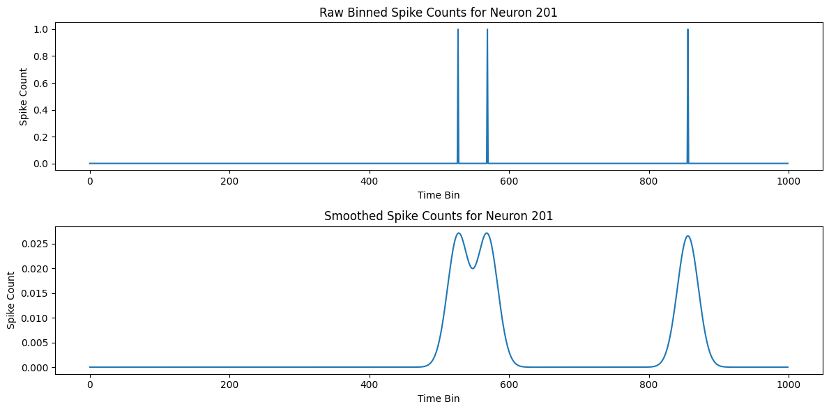
Smoothing
The raw binned data can be quite noisy, as it includes both the signal (the underlying neural activity) and the noise (random fluctuations). Smoothing can help reduce this noise and make the signal more apparent. One common way to smooth the data is to convolve it with a Gaussian kernel. This is equivalent to replacing each spike count with a weighted average of the spike counts in nearby time bins, where the weights are determined by a Gaussian function. This has the effect of smoothing out rapid fluctuations in the spike counts.
After initial binning and smoothing, we get the data \(X\) in an \(M \times{N}\) matrix format where \(N\) is the number of neurons and the \(M\) is the fixed length time dimension.
Given this format, the neural population activity at any given point in time \(t\) can be plotted in this \(N\)-dimensional space that is spanned by the \(N\) number of neurons. So each sample in this matrix \(X\) is a point in this \(N\)-dimensional space.
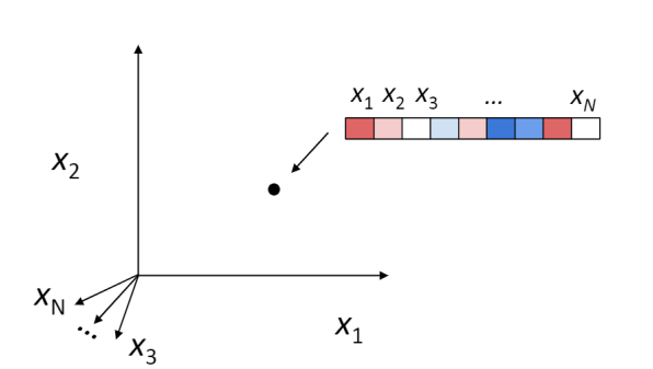
If we were to plot the recorded neuronal population activity in this \(N\)-dimensional space within a certain time interval, one might hypothesize that the neurons will explore the whole space. But this is not the case.
It has been shown through several repeated experiments that a population of neurons does not explore the whole high \(N\)-dimensional space. Instead, due to the fact that these neurons are interconnected to each other and are not entirely independent, their overall activity is confined to a lower dimensional subspace residing in this high dimensional space. These subspaces are often referred to as Neural Manifolds.

These Neural Manifolds can be uncovered with dimensionality reduction techniques like PCA. The idea is to reduce the dimensionality of the data and to identify these main modes of variation in the neural activity.
The Manifolds are spanned by these Neural Modes. These modes capture the coordinated activity among neurons that often underlie specific functions or behaviors.
Principle Component Analysis
Principal Component Analysis (PCA) is a statistical procedure that uses an orthogonal transformation to convert a set of observations of possibly correlated variables into a set of values of linearly uncorrelated variables called principal components. This transformation is defined in such a way that the first principal component has the largest possible variance (that is, accounts for as much of the variability in the data as possible), and each succeeding component in turn has the highest variance possible under the constraint that it is orthogonal to the preceding components. The resulting vectors are an uncorrelated orthogonal basis set.
In other words, the Principal components are basically the orthogonal neural modes. When the original neural population activity is projected onto these neural modes (Principal components), they reveal the underlying pattern of activity. Since the results of projecting the neural activity onto a neural mode is basically equivalent to finding the weighted linear combination of the original neurons that shows their contribution to that specific mode.
Now, let’s dive a bit deeper into the mathematics of PCA.
Sticking to our previous notation for the neural data. Given a dataset \(X\) of dimension \(M \times N\) (where \(M\) is the number of observations and \(N\) is the number of variables), the goal of PCA is to find a new set of variables, the principal components, that are uncorrelated and that explain the most variance. In other words, we want to find a new basis for the data that retains the most information. In machine learning terms, the \(M\) observations are the samples and the \(N\) variables are the features. The principal components are the new features that we want to find.
Note: In case of our neural data, our observations (\(N\)) are the neurons and the and each value across \(M\) is the activity of a certain neuron at a certain time point. According to the hypothesis we established earlier, the neural activity is confined to a lower dimensional manifold. So, the principal components are the new features that we want to find that span this \(d\)-dimensional manifold such that \(d < N\). Implying that the neural population activity can be explained with a lower number of hidden variables (refer to as neural modes) instead of the original \(N\) neurons.
The first step in PCA is to standardize the data. This involves subtracting the mean and dividing by the standard deviation for each variable. Let’s denote the standardized data as \(Z\).
The next step is to compute the covariance matrix of \(Z\). The covariance matrix \(C\) is given by:
\[C = \frac{1}{N-1} Z^T Z\]The covariance matrix is a symmetric matrix that contains the variances of the variables on its diagonal and the covariances between each pair of variables in the other entries.
The next step is to compute the eigenvalues and eigenvectors of the covariance matrix. The eigenvectors of the covariance matrix correspond to the principal components and the eigenvalues correspond to the variance explained by the principal components.
Let’s denote the eigenvalues by \(\lambda_i\) and the eigenvectors by \(v_i\). They satisfy the following equation:
\[C v_i = \lambda_i v_i\]The principal components are then given by projecting the standardized data \(Z\) onto the eigenvectors:
\[PC_i = Z v_i\]The variance explained by the \(i\) th principal component is given by the corresponding eigenvalue \(\lambda_i\).
Let’s denote our data matrix as \(X\), where each row corresponds to a single time point and each column corresponds to a single neuron. After preprocessing and standardizing our data, we perform PCA on \(X\).
The PCA procedure will yield a set of eigenvectors \(v_i\) (the principal components) and corresponding eigenvalues \(\lambda_i\). Each eigenvector \(v_i\) is a vector of the same length as the number of neurons, and its elements are the coefficients of the linear combination of the original neurons’ activities that forms the principal component.
So, if we have \(N\) neurons, each eigenvector \(v_i\) will be a \(N\)-dimensional vector, where the \(j\)th element of \(v_i\) represents the contribution of the \(j\)th neuron to the \(i\)th principal component.
To be more explicit, if \(v_i = [c_1, c_2, ..., c_N]\) is the \(i\)th principal component, then the \(i\)th principal component is a linear combination of the original neurons given by:
\[PC_i = c_1 * neuron_1 + c_2 * neuron_2 + ... + c_N * neuron_N\]where \(c_j\) is the contribution (or weight) of the \(j\) th neuron to the \(i\) th principal component, and \(neuron_j\) is the activity of the \(j\) th neuron.
These weights \(c_j\) can be positive or negative, and their magnitude indicates the degree to which each neuron contributes to the principal component. A large positive weight means that the neuron strongly contributes to the principal component, while a large negative weight means that the neuron contributes in the opposite direction. A weight close to zero means that the neuron does not contribute much to the principal component.
Note: The goal of apply PCA is to achieve dimetionality reduction across the neurons and NOT the time points.
Let’s consider our original neural dataset \(X\) of dimension \(M \times N\) , where \(N\) is the number of neurons and \(M\) is the number of observations (time points). The data matrix \(X\) can be written as:
\[X = [x_1, x_2, ..., x_N] = \begin{bmatrix} x_{11} & x_{12} & \cdots & x_{1N} \\ x_{21} & x_{22} & \cdots & x_{2N} \\ \vdots & \vdots & \ddots & \vdots \\ x_{M1} & x_{M2} & \cdots & x_{MN} \end{bmatrix}\]where \(x_{ij}\) is the activity at the \(i\) th time pooint of the \(j\) th neuron time point.
After applying PCA, we obtain a set of principal components. Let’s denote the first three principal components as \(v_1\) , \(v_2\) , and \(v_3\) . Each of these is a vector of length \(M\) , so they can be written as:
\(v_1 = [v_{11}, v_{12}, ..., v_{1N}]^T\)
\(v_2 = [v_{21}, v_{22}, ..., v_{2N}]^T\)
\(v_3 = [v_{31}, v_{32}, ..., v_{3N}]^T\)
Here, \(v_{ij}\) is the contribution of the \(j\) th neuron to the \(i\) th principal component or neural mode.
These principal components can be combined into a \(3 \times N\) matrix \(V\) , where each row is a principal component:
\[V = [v_1^T; v_2^T; v_3^T] = \begin{bmatrix} v_{11} & v_{12} & \cdots & v_{1N} \\ v_{21} & v_{22} & \cdots & v_{2N} \\ v_{31} & v_{32} & \cdots & v_{3N} \end{bmatrix}\]The activation dynamics of the principal components can be computed by projecting the original data onto the principal components. This can be done via matrix multiplication:
\[A = XV^T\]Here, \(A\) is a \(M \times 3\) matrix, where each column is the activation dynamics of a principal component:
\[A = [a_1, a_2, a_3] = \begin{bmatrix} a_{11} & a_{21} & a_{31} \\ a_{12} & a_{22} & a_{32} \\ \vdots & \vdots & \vdots \\ a_{M1} & a_{M2} & a_{M3} \end{bmatrix}\]Here, \(a_{ij}\) is the activation of the \(i\) th principal component for the \(j\) th neuron.
So, the matrix \(V\) represents the principal components in the space of the original time points, and the matrix \(A\) represents the activation dynamics of the principal components for each neuron.
The original neuron activity can be reconstructed from the principal components by reversing the projection. This can be done via matrix multiplication:
\[X_{recons} = AV\]Here, \(X_{recons}\) is a \(M \times N\) matrix, where each column is the recons activity of a neuron:
\[X_{recons} = \\ [x_{recons,1}, x_{recons,2}, ..., x_{recons,M}] = \\ \begin{bmatrix} x_{recons,11} & x_{recons,12} & \cdots & x_{recons,1N} \\ x_{recons,21} & x_{recons,22} & \cdots & x_{recons,2N} \\ \vdots & \vdots & \ddots & \vdots \\ x_{recons,M1} & x_{recons,M2} & \cdots & x_{recons,MN} \end{bmatrix}\]Here, \(x_{recons,ij}\) is the reconstructed activity of the \(i\) th neuron at the \(j\) th time point.
This is how you can interpret the principal components representing the neural modes that are computed as the linear combinations of the original neurons and how the original neural activity can be represented as the linear combination of the activation dynamics \(A\) and the neural modes or eigen matrix \(V\)
Now let’s implement this in python.
#@title Data retrieval
#@markdown This cell downloads the example dataset that we will use in this tutorial.
import io
import requests
import numpy as np
r = requests.get('https://osf.io/sy5xt/download')
if r.status_code != 200:
  print('Failed to download data')
else:
  spike_times = np.load(io.BytesIO(r.content), allow_pickle=True)['spike_times']
spike_times.shape
(734,)
# Define the bin edges (for example, bins of 1 millisecond from 0 to the maximum spike time)
bin_edges = np.arange(0, np.max([np.max(st) for st in spike_times]), 0.001)

# Initialize an empty array to hold the binned data
binned_data = np.zeros((len(bin_edges)-1, len(spike_times)))

# For each neuron, count the number of spikes in each bin
for i, neuron_spike_times in enumerate(spike_times):
    binned_data[:, i], _ = np.histogram(neuron_spike_times, bins=bin_edges)
from scipy.ndimage import gaussian_filter1d

# Apply a Gaussian filter to each neuron's binned spike counts
smoothed_data = gaussian_filter1d(binned_data[:50000, :], sigma=15, axis=0)
smoothed_data.shape
(50000, 734)
import matplotlib.pyplot as plt

# Choose a neuron to visualize
neuron = 200

# Plot the raw binned spike counts
plt.figure(figsize=(12, 6))
plt.subplot(2, 1, 1)
plt.plot(binned_data[:1000, neuron])
plt.title('Raw Binned Spike Counts for Neuron {}'.format(neuron+1))
plt.xlabel('Time Bin')
plt.ylabel('Spike Count')

# Plot the smoothed spike counts
plt.subplot(2, 1, 2)
plt.plot(smoothed_data[:1000, neuron])
plt.title('Smoothed Spike Counts for Neuron {}'.format(neuron+1))
plt.xlabel('Time Bin')
plt.ylabel('Spike Count')

plt.tight_layout()
plt.show()
smoothed_data[:, :100].shape
(50000, 100)
from sklearn.decomposition import PCA

# Apply PCA
pca = PCA()
pca.fit(smoothed_data[:, :])

# Transform the data into the principal component space
smoothed_data_pca = pca.transform(smoothed_data[:, :])
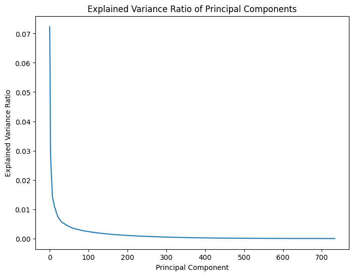
plt.figure(figsize=(8, 6))

plt.plot(pca.explained_variance_ratio_)
plt.title('Explained Variance Ratio of Principal Components')
plt.xlabel('Principal Component')
plt.ylabel('Explained Variance Ratio')

plt.show()
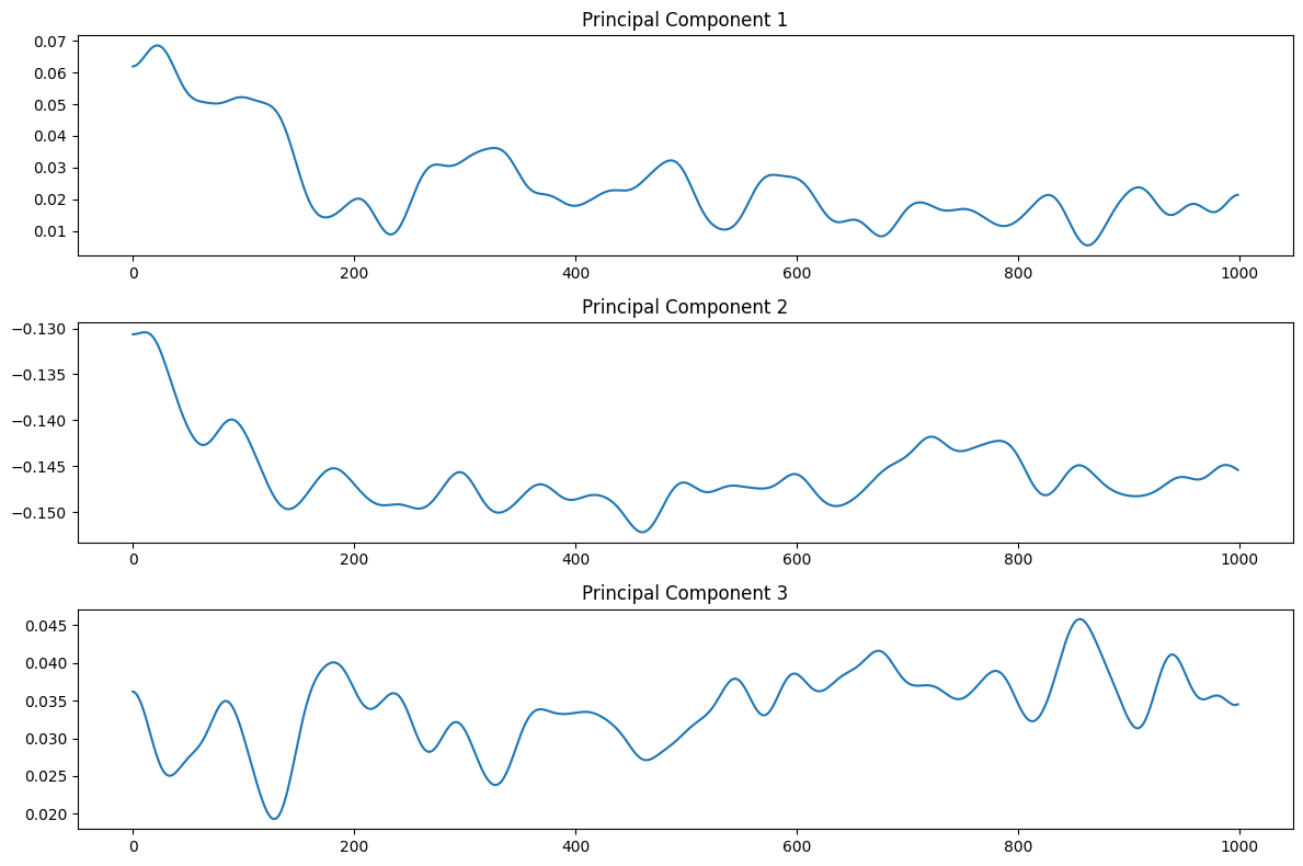
plt.figure(figsize=(12, 8))

for i in range(3):
    plt.subplot(3, 1, i+1)
    plt.plot(smoothed_data_pca[:1000, i])
    plt.title(f'Principal Component {i+1}')

plt.tight_layout()
plt.show()
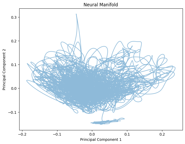
plt.figure(figsize=(8, 6))

plt.plot(smoothed_data_pca[:, 0], smoothed_data_pca[:, 1], alpha=0.5)
plt.xlabel('Principal Component 1')
plt.ylabel('Principal Component 2')
plt.title('Neural Manifold')

plt.show()
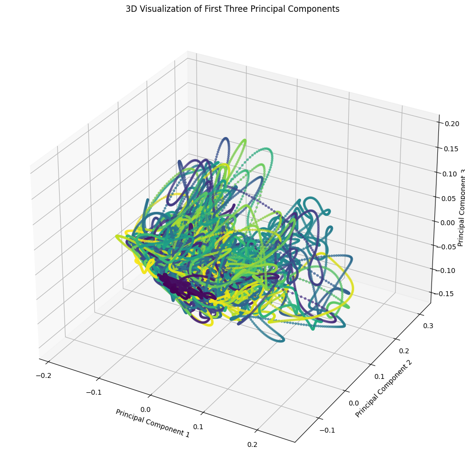
%matplotlib inline


fig = plt.figure(figsize=(15, 12))
ax = fig.add_subplot(111, projection='3d')

# Create a sequence of colors based on time
colors = plt.cm.viridis(np.linspace(0, 1, smoothed_data_pca.shape[0]))

# Plot a line in 3D space
ax.plot(smoothed_data_pca[:, 0], smoothed_data_pca[:, 1], smoothed_data_pca[:, 2], color='darkblue', alpha=0.6, lw=0.5)
# Plot points along the line
ax.scatter(smoothed_data_pca[:, 0], smoothed_data_pca[:, 1], smoothed_data_pca[:, 2], c=colors, alpha=0.6, s=8)

ax.set_xlabel('Principal Component 1')
ax.set_ylabel('Principal Component 2')
ax.set_zlabel('Principal Component 3')
ax.set_title('3D Visualization of First Three Principal Components')

plt.show()
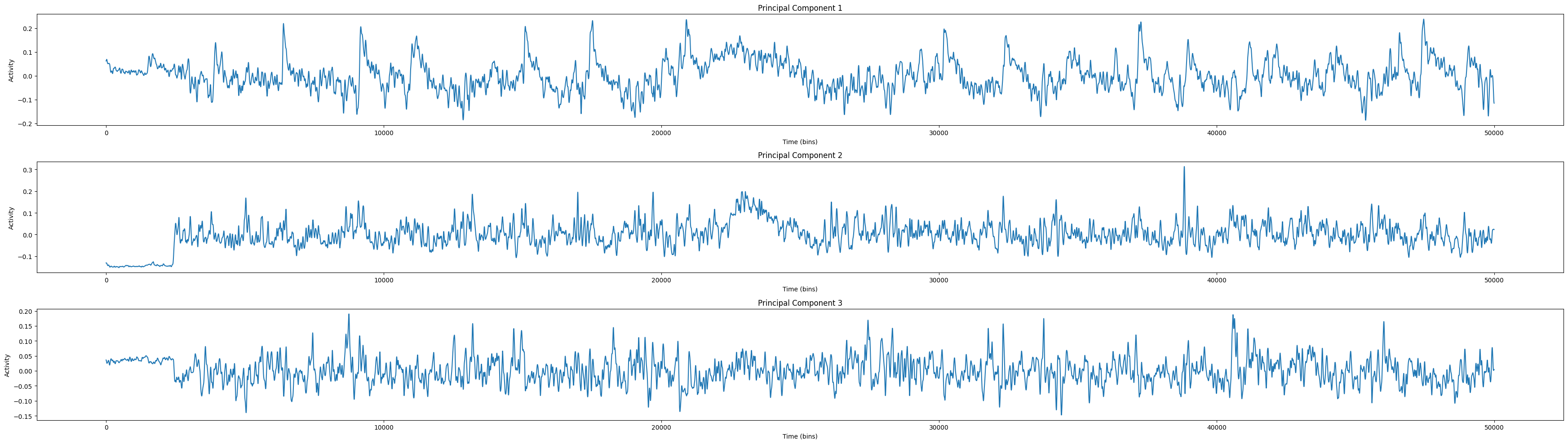
import matplotlib.pyplot as plt

# Define the number of principal components to plot
num_components = 3

plt.figure(figsize=(35, 10))

# Plot each principal component
for i in range(num_components):
    plt.subplot(num_components, 1, i+1)
    plt.plot(smoothed_data_pca[:, i])
    plt.title(f'Principal Component {i+1}')
    plt.xlabel('Time (bins)')
    plt.ylabel('Activity')

plt.tight_layout()
plt.show()
Conclusion
Applying PCA to neural data, which is essentially time series data, is a common practice in neuroscience. The idea is to reduce the dimensionality of the data and to identify the main modes of variation in the neural activity. Here’s how it can be done
Preprocessing: Neural data often needs to be preprocessed before PCA can be applied. This can involve steps like filtering the data to remove noise, normalizing the data, or subtracting the mean activity across all neurons.
Formatting the data: For PCA, the data needs to be in a 2D matrix format, where each row is an observation and each column is a variable. In the context of neural data, an observation could be the activity of all neurons at a single point in time, and a variable would be the activity of a single neuron over time. So, you would reshape your data such that each row of your matrix corresponds to a single time point, and each column corresponds to a single neuron.
Applying PCA: Once your data is in the correct format, you can apply PCA as usual. This involves computing the covariance matrix of your data, and then finding the eigenvalues and eigenvectors of this matrix. The eigenvectors are the principal components, and they represent the directions in which your data varies the most.
Interpreting the results: The output of PCA will be a set of principal components, which are orthogonal to each other and explain the maximum variance in the data. Each principal component is a linear combination of the original neurons, and the coefficients in this linear combination tell you how much each neuron contributes to that component. The first few principal components often capture a large portion of the variance in the data, and can be used to visualize and further analyze the data.
It’s important to note that PCA is a linear method, which means it assumes that the main modes of variation in your data are linear. If this is not the case, other methods like Independent Component Analysis (ICA) or Non-negative Matrix Factorization (NMF) might be more appropriate.
Also, PCA does not take into account the temporal structure of the data. If the temporal dynamics are important, methods like time-lagged PCA or dynamical systems analysis might be more appropriate.
Share on
Twitter Facebook LinkedInComments are configured with provider: facebook, but are disabled in non-production environments.